Turbofan Engine RUL Prediction

View on GitHub →

1- Overview

An end-to-end predictive maintenance system for aircraft turbofan engines. RUL prediction on NASA CMAPSS dataset using Random Forest, XGBoost, sklearn Pipelines & MLflow.

---

2- Context & Motivation

Problem Statement

Aviation maintenance operates on two modes: scheduled (replace every N hours regardless of condition) and unscheduled (repair after failure). The first wastes money by replacing healthy components while the second risks catastrophic in-flight failure. Predictive maintenance is the third way: maintenance operations are scheduled when and only when a component is approaching failure.

The business case is substantial: a single unplanned engine removal can rapidly cost hundreds of thousands of dollars in AOG (Aircraft on Ground)fees and emergency parts, before even accounting for safety consequences.

Technical challenges

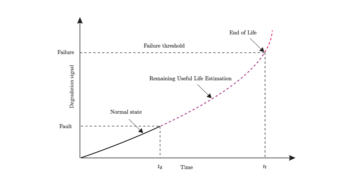
An aircraft turbofan engine degrades continuously through thousands of operational cycles. The challenge is to:

• Extract a clean degradation signal from noisy, high-dimensional time-series data
• Predict the number of remaining cycles with sufficient accuracy to schedule maintenance in advance
• Generalize to engines the model has never observed

To do so, RUL (Remaining Useful Life) is introduced. Predicting it accurately is the key challenge in maintenance prediction problems, and can be applied to a broad range of scientific and industrial applications.

Project Goal & Methodology

Build an end-to-end ML pipeline from raw sensor data to operational risk assessment, using the NASA CMAPSS benchmark dataset, validated against the official NASA test set and the PHM 2008 competition scoring function.

3- Dataset

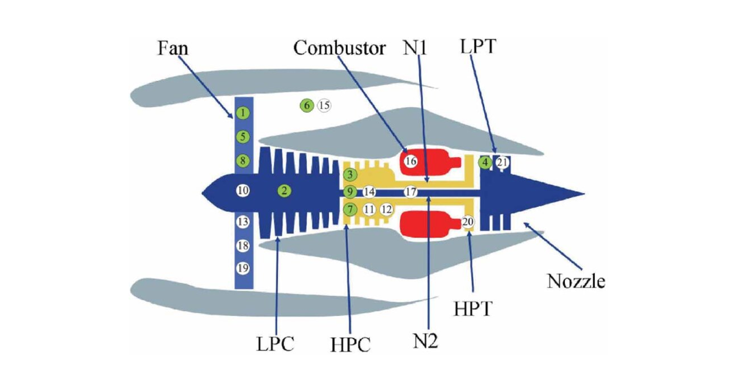
CMAPSS (Commercial Modular Aero-Propulsion System Simulation) was released by NASA Ames Research Center for the 2008 PHM challenge and remains the standard benchmark for RUL prediction. It simulates run-to-failure degradation of a turbofan engine’s high-pressure compressor.

This project uses the FD001 subset: 100 training engines and 100 test engines, all operating under a single condition with a single fault mode.

Each row in the dataset represents one engine at one operational cycle, with 21 sensor readings and 3 operating condition settings:

#	Symbol	Description	Unit
Engine
Cycle
Setting 1		Altitude	ft
Setting 2		Mach Number	M
Setting 3		TRA (Throttle-Resolver Angle)	deg
Sensor 1	T2	Total temperature at fan inlet	°R
Sensor 2	T24	Total temperature at LPC outlet	°R
Sensor 3	T30	Total temperature at HPC outlet	°R
Sensor 4	T50	Total temperature at LPT outlet	°R
Sensor 5	P2	Pressure at fan inlet	psia
Sensor 6	P15	Total pressure in bypass-duct	psia
Sensor 7	P30	Total pressure at HPC outlet	psia
Sensor 8	Nf	Physical fan speed	rpm
Sensor 9	Nc	Physical core speed	rpm
Sensor 10	epr	Engine pressure ratio	–
Sensor 11	Ps30	Static pressure at HPC outlet	psia
Sensor 12	phi	Ratio of fuel flow to Ps30	pps/psi
Sensor 13	NRf	Corrected fan speed	rpm
Sensor 14	NRc	Corrected core speed	rpm
Sensor 15	BPR	Bypass ratio	–
Sensor 16	farB	Burner fuel-air ratio	–
Sensor 17	htBleed	Bleed enthalpy	–
Sensor 18	Nf_dmd	Demanded fan speed	rpm
Sensor 19	PCNfR_dmd	Demanded corrected fan speed	rpm
Sensor 20	W31	HPT coolant bleed	lbm/s
Sensor 21	W32	LPT coolant bleed	lbm/s

• LPC/HPC: Low/High Pressure Compressor
• LPT/HPT: Low/High Pressure Turbine

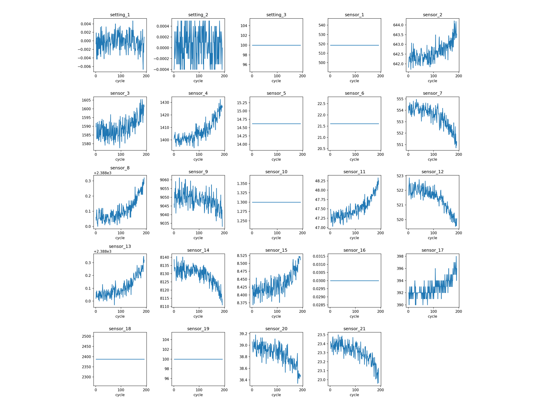
Engine 1 sensors show a clear monotonic degradation while others are flat or pure noise:

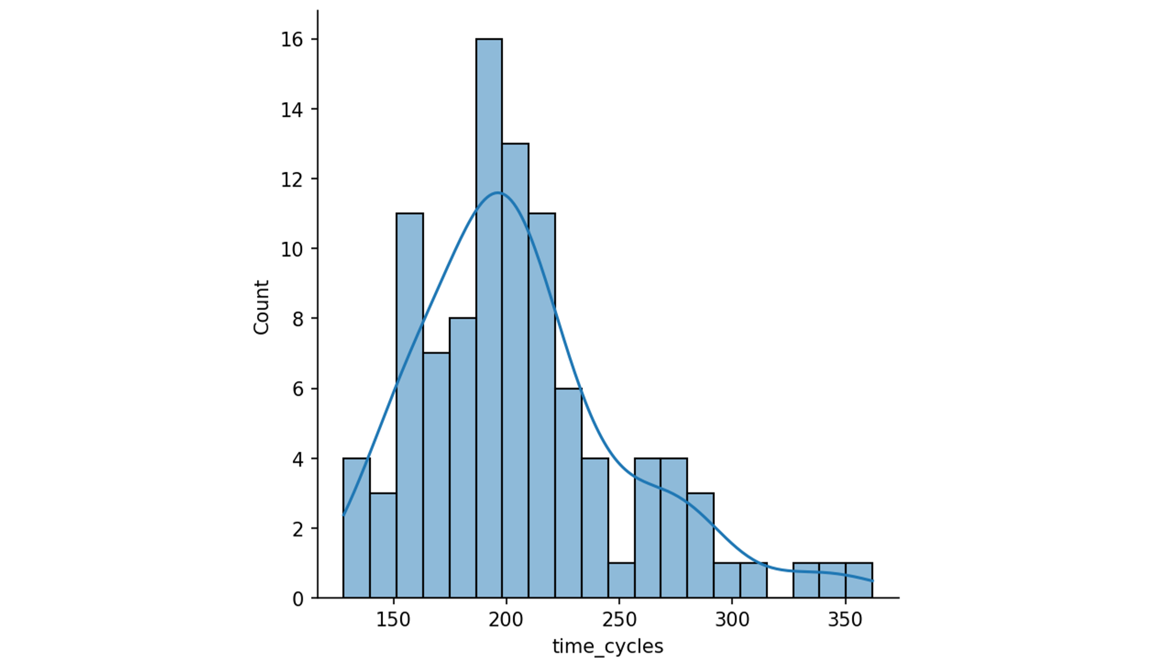
Engine lifetimes in the training set range from 128 to 362 cycles, giving the following distribution:

---

4- Feature Engineering

Raw sensor readings require significant transformation before they can be used as model inputs. Four operations are applied in sequence:

RUL computation and clipping

For each engine: $$\text{RUL}(t) = \text{max\_cycles} - t$$

A clip of 120 cycles is applied. Beyond this value, the engine is healthy and predicting a precise RUL has less operational relevance. Indeed, maintenance is not scheduled 300 cycles in advance. This clipping is standard in the CMAPSS literature and also speeds up convergence so that the model focuses on the region where prediction matters.

Low-variance feature removal

Features whose variance falls below $10^{-5}$ are constant (or near-constant) and carry no useful information.

Temporal features

Mechanical degradation is a slow process. In order to capture underlying trends while smoothing the noise, a 5-cycle rolling mean and standard deviation are implemented, as well as an instantaneous difference to capture rapid changes. For each retained sensor we then get:

• rolling_mean_5 for local trend
• rolling_std_5 for local variability
• diff_1 (first-order difference) for the rate of change

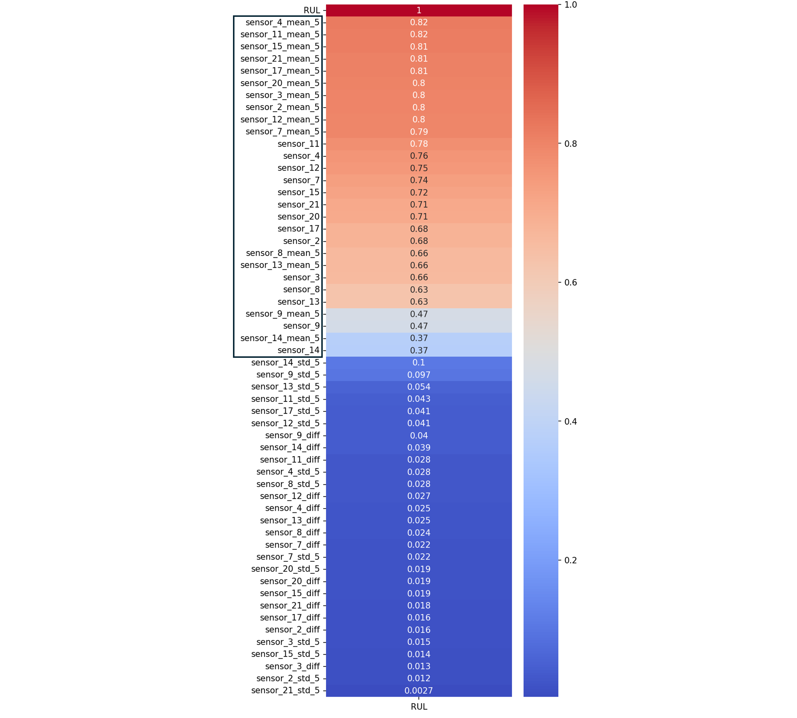
Correlation filtering

Features with $|\text{corr}(\text{RUL})| \leq 0.1$ are removed. The final feature set contains 28 features.

---

5- Model Selection & Training

The split is performed by engine unit (not randomly across rows) to prevent data leakage: the same engine can’t appear in both training and test sets. A standard progression from simple to more complex models is then followed.

Baseline

The baseline model systematically predicts the mean RUL of the training set for every observation. It is the minimum benchmark to outperform.

Linear Regression

First supervised model, scale-sensitive so wrapped in a StandardScaler, to discover if the degradation signal is partially linearly exploitable.

Random Forest

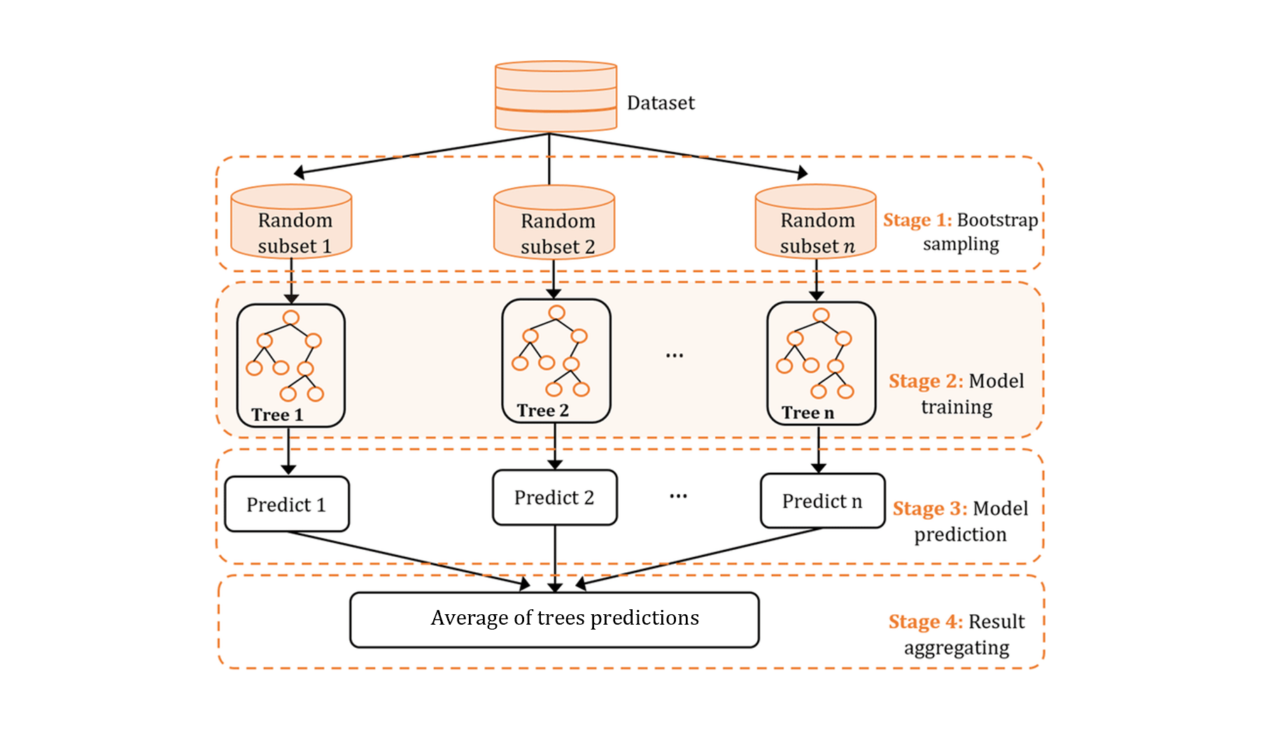
As a reminder, Random Forest is an ensemble learning model of decision trees, each trained on a random subset of features and data (bagging). The final prediction is the average across all trees. Each tree sees a random bootstrap sample of the data and at each split considers only a random subset of features. This double randomness reduces variance (overfitting) while keeping each tree individually interpretable.

Before hyperparameter tuning, a vanilla Random Forest is trained with default parameters, and the top 15 features by importance are selected. Feature importance is measured by average impurity decrease (Gini) across all splits — providing interpretable feature rankings. Reducing dimensionality at this stage lowers overfitting and speeds up the grid search.

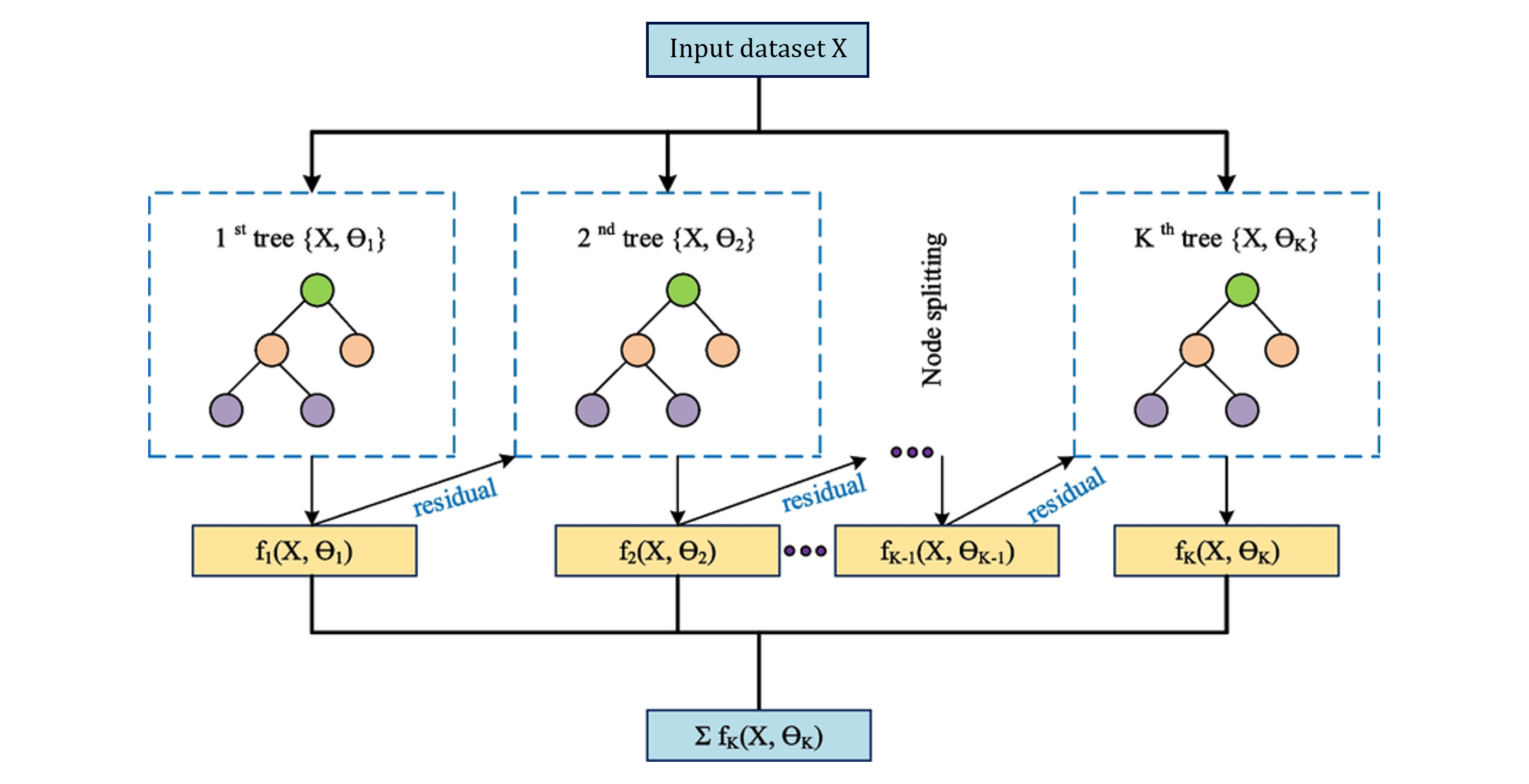
XGBoost

Gradient-boosted trees: rather than building trees in parallel (like RF), XGBoost builds them sequentially, each tree correcting the residual errors of the previous. This makes it more data-efficient, but also more prone to overfitting without regularization.

Before hyperparameter tuning, a vanilla XGBoost is trained with default parameters, and the top 15 features by importance are selected. XGBoost uses gain-based feature importance (improvement in loss from each split), which ranks features differently than RF’s Gini impurity.

Hyperparameter tuning (Random Forest and XGBoost)

GridSearchCV() over the key regularization parameters:

Model	Parameters tuned
Random Forest	n_estimators ∈ {100, 200, 300}
	max_depth ∈ {None, 10, 20}
	min_samples_leaf ∈ {1, 3, 5}
XGBoost	n_estimators ∈ {100, 200, 300}
	max_depth ∈ {3, 5, 7}
	learning_rate ∈ {0.05, 0.1, 0.2}

Preventing data leakage with GroupKFold for cross-validation

A random train/test split would place different cycles of the same engine in both train and test folds. GroupKFold partitions by engine unit, ensuring each fold contains engines unseen during training, therefore avoiding any data leakage.

---

6- Results

Each model is wrapped in a sklearn Pipeline (scaler → model). MLflow experiment tracking is implemented and enables direct run comparison in the MLflow UI.

Metrics (RMSE, MAE, R², NASA Score)

Standard regression metrics for model selection: $$ \mathbf{RMSE} = \sqrt{\frac{1}{n} \sum_{i=1}^{n} (y_i - \hat{y}_i)^2} $$ $$ \mathbf{MAE} = \frac{1}{n} \sum_{i=1}^{n} |y_i - \hat{y}_i| $$ $$ \mathbf{R^2} = 1 - \frac{\sum_{i=1}^{n} (y_i - \hat{y}_i)^2} {\sum_{i=1}^{n} (y_i - \bar{y})^2} $$

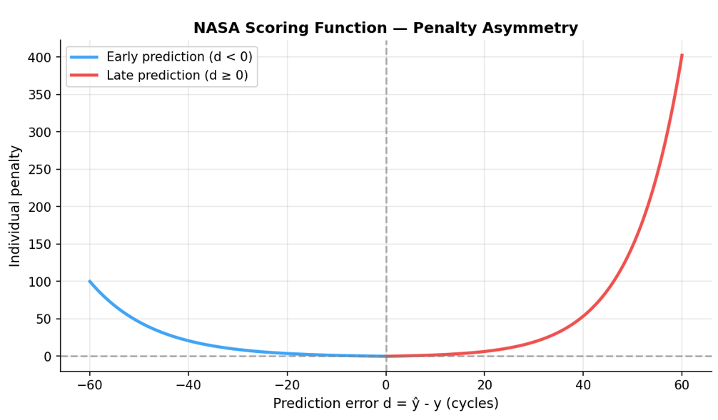
In addition, the NASA asymmetric scoring function for operational validation is introduced.

For each engine, the individual score is:

$$s_i = \begin{cases} e^{-d_i/13} - 1 & \text{if } d_i < 0 \text{ (early prediction)} \\ e^{d_i/10} - 1 & \text{if } d_i \geq 0 \text{ (late prediction)} \end{cases}$$

where $d_i = \hat{y}_i - y_i$ is the prediction error.

The total score is $S = \sum_i s_i$. Lower is better, an undetected failure is far more costly than a preventive maintenance action.

Model comparison

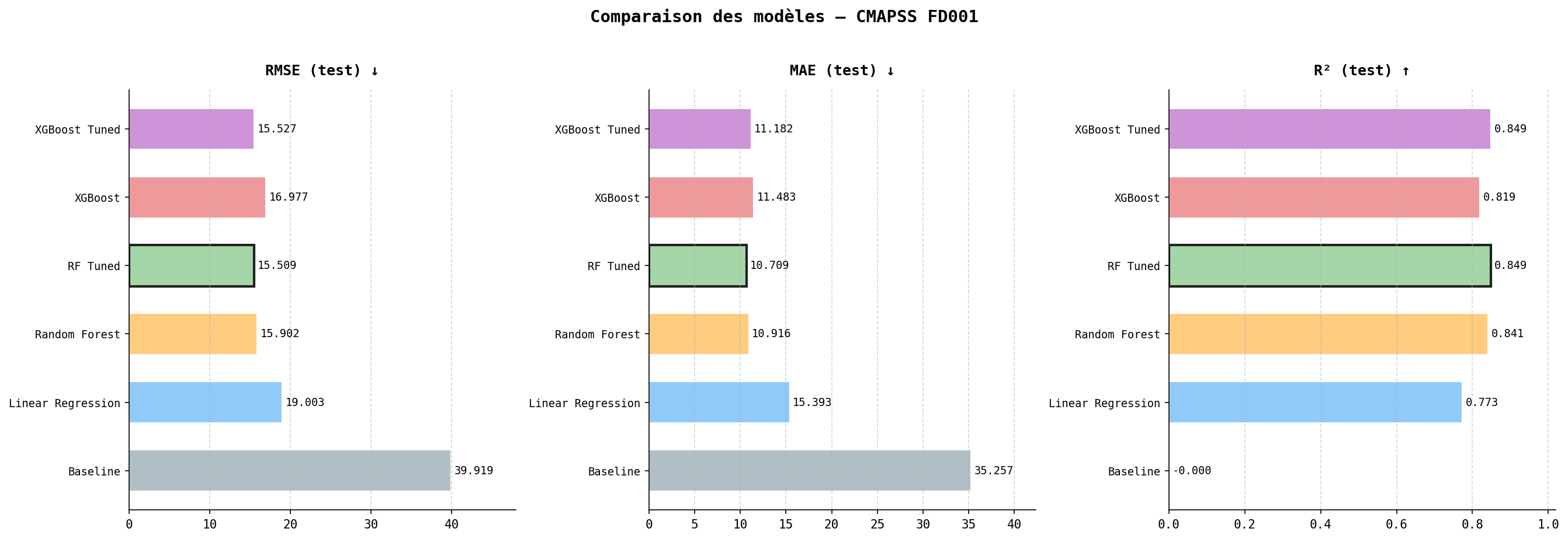
Model	RMSE (test)	MAE (test)	R² (test)
Baseline	39.92	35.26	0.000
Linear Regression	19.00	15.39	0.773
Random Forest	15.90	10.92	0.841
RF Tuned	15.51	10.71	0.849
XGBoost	16.98	11.48	0.819
XGBoost Tuned	15.53	11.18	0.849

Tuning narrows the train/test gap substantially in both RF and XGBoost, confirming the initial vanilla models were overfitting. RF Tuned and XGBoost Tuned reach essentially identical performance. Random Forest Tuned model is selected as the final model for its robustness and interpretability.

NASA benchmark

The final model is retrained on the full training set and evaluated on the official NASA test file, a completely held-out set never seen during development.

Metric	Value
RMSE	17.34 cycles
MAE	12.10 cycles
R²	0.806
NASA Score	902.7

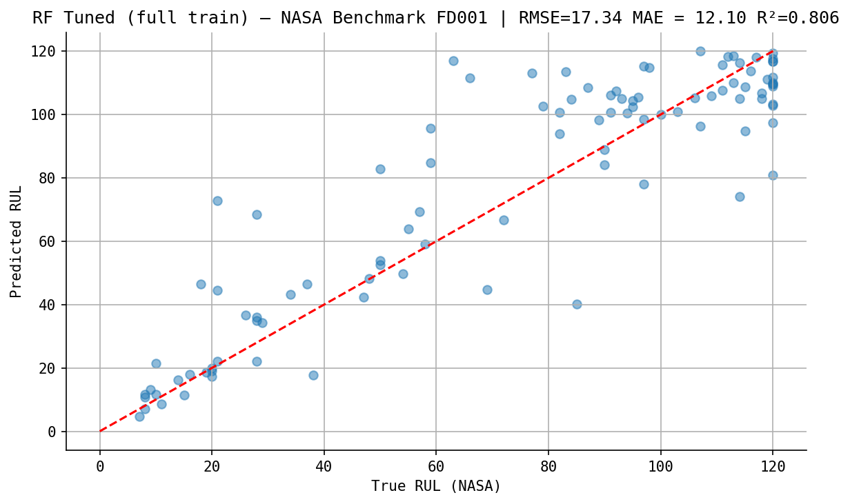
A NASA score of 902.7 is an encouraging result, ranking our model among the top 6 (based on the PHM 2008 competition results). However, this should be interpreted with caution, as we only used the FD001 dataset, which is the easiest subset.

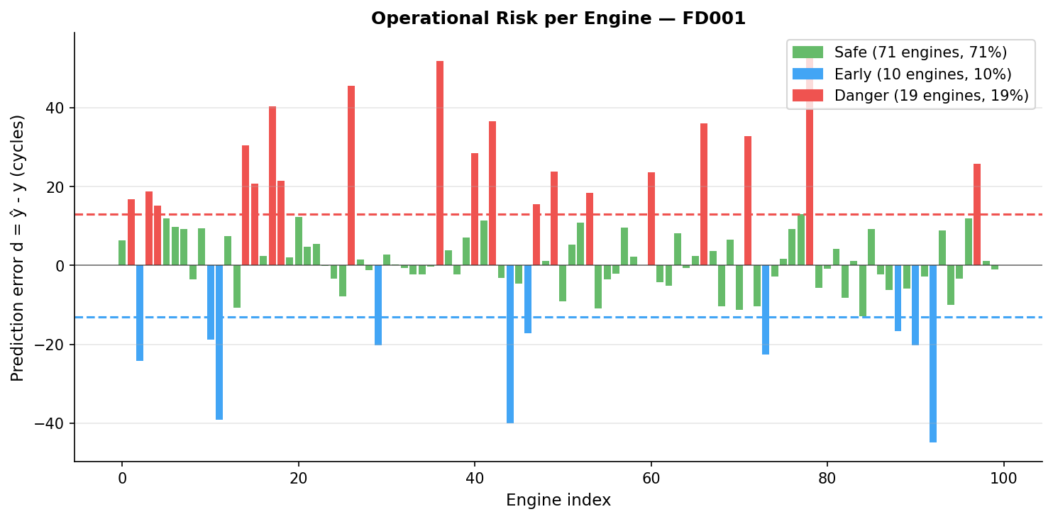
Operational risk analysis

In a real maintenance context, maintenance is triggered when the predicted RUL falls below an operational threshold, determined by a human operator. For aerospace applications, the threshold should be set conservatively low given the catastrophic cost of an in-flight failure.

To translate our model performance into business value, we categorize predictions into three operational zones:

Zone	Condition	Operational consequence
Safe	$ abs(d) <= 13 $ cycles	Maintenance planned correctly
Early warning	$d < -13$ cycles	Unnecessary early intervention
Danger	$d > 13$ cycles	Engine may fail before maintenance, critical safety risk

The threshold of 13 cycles is derived from the NASA scoring function scale parameter for early predictions.

---

7- Conclusion & Next Steps

Physical Interpretation

T50 (LPT outlet temperature) emerges as the dominant predictor of RUL. This result aligns with FD001 dataset single fault mode. Because T50 sits at the very end of the gas path, it acts as a natural integrator of all upstream degradation mechanisms, making it the most informative single signal for RUL estimation.

The use of a 5-cycle rolling mean across all selected features is physically motivated: mechanical degradation is a slow, cumulative process whose signature is more reliably captured over several consecutive cycles than in any instantaneous measurement.

Limitations and next steps

• FD001 is the simplest CMAPSS subset: single operating condition, single fault mode. Extending to FD002/FD003/FD004 (multiple conditions, multiple fault modes) would better reflect real-world complexity.

• The RUL clipping at 120 cycles is a modeling assumption. In production, a two-stage model could first classify whether the engine is in its degradation phase before predicting RUL.

• LSTM / Transformer architectures are known to outperform classical ML models on this benchmark by explicitly modeling temporal dependencies, this is what I will focus on next.

---

Python · pandas · numpy · scikit-learn · sklearn Pipeline · XGBoost · MLFlow · matplotlib · seaborn · joblib