
View full report (PDF) →View on GitHub →
1- Overview
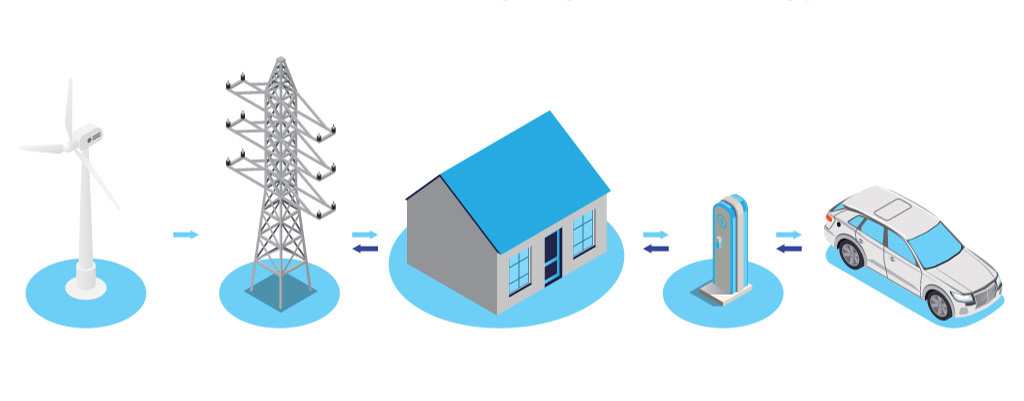
Intelligent electric vehicle charging optimization using LSTM emission forecasting and convex optimization to minimize CO2 emissions while ensuring user mobility needs.
2- Context & Motivation
Problem Statement
The rapid adoption of electric vehicles represents a critical strategy for addressing energy dependence and mitigating climate change. As EV adoption accelerates, a new challenge emerges: the growing strain on the energy grid. The current infrastructure is already stressed by rising energy demand, and this demand will only intensify as EV adoption becomes widespread.
The challenge manifests in two distinct charging infrastructure needs: public charging stations and residential home chargers. This project focuses exclusively on home charging, as public stations operate on a fast-charging model where drivers top up quickly, leaving minimal room for optimizing the power delivery curve.
The core inefficiency: Home charging typically occurs overnight when users plug in after returning home. This creates two critical problems:
- Peak grid demand - simultaneous evening charging (5-10pm) creates a second daily peak, risking grid overload
- Maximum emissions - nighttime charging coincides with the absence of solar energy, forcing reliance on high-carbon generation sources (800-1000 lbs CO2/MWh vs. 50 lbs during solar windows)
Not every vehicle requires 100% charge daily. The median commute requires only 20-30% SOC replenishment, yet standard practice charges to full capacity regardless of actual need.
Technical Challenge
The need for dynamic charging policy stems from a fundamental mismatch between user behavior (plug in at night, charge to 100%) and grid reality (electricity is dirtiest at night, most users don’t need full charge).
To prescribe an optimal charging policy, three interdependent challenges must be solved:
1. Emission forecasting
Predict the Marginal Operating Emission Rate (MOER) - CO2 lbs/MWh at 5-minute intervals - for the next 24 hours. Challenge: unpredictable daily spikes in emission data. Summer patterns are consistent (reliable solar windows), but winter spikes occur randomly due to inconsistent weather (cloud cover, rainfall, snow).
2. Battery modeling
Derive accurate power-SOC relationships that capture the battery’s non-linear voltage behavior across the full charge range. The model must be convex (solvable by optimization algorithms) while remaining physically realistic.
3. Real charging constraints
Honor actual user charging patterns from empirical data: plug-in/plug-out times, required final SOC, session duration. Simulated driving behavior fails to capture real-world variability.
Project Goal
Create an optimized charging policy that:
- Charges opportunistically during low-emission windows
- Charges only to the SOC needed for the next trip (plus safety buffer)
- Reduces grid load during peak hours
This approach addresses both environmental impact (minimize emissions) and grid stability (flatten demand curve), while ensuring user mobility needs are met.
3- Data Sources
This project integrates three datasets: emission time-series, battery electrochemistry simulations, and real residential charging sessions.
Emission Curve Data
CAISO North Marginal Operating Emission Rate (MOER) from WattTime API
Time-series of CO2 lbs/MWh at 5-minute intervals for Northern California (1 full year). MOER represents the marginal emissions from the next unit of electricity generation.
Battery Data
PyBamm Single Particle Model is used to simulate a Tesla Model 3 Long Range battery pack of 4,416 cells (96 series × 46 parallel):
| Parameter | Tesla cell | PyBamm Model |
|---|---|---|
| Capacity | 4.8 Ah | 4.73 Ah |
| Lower cutoff | 2.5 V | 2.6 V |
| Upper cutoff | 4.2 V | 4.1 V |
Charging Session Data
Simulated driving surveys (NHTS) assume uniform behavior and neglect the high variability captured by real-world data (weekend vs weekday, irregular plug-in times). Real residential charging dataset from a Norway housing cooperative is therefore used:
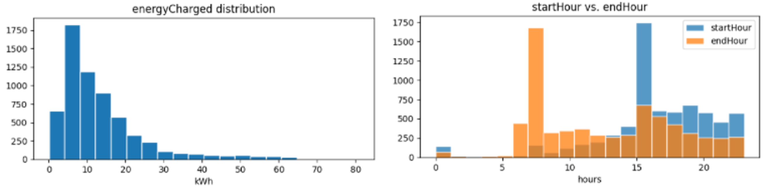
6,844 sessions from 96 users (Dec 2018 – Jan 2020). Each session records plug-in/plug-out timestamp, energy charged (kWh) and user ID.
| Statistic | Value |
|---|---|
| Avg plug-in duration | 11.85 hours |
| Avg energy charged | 15.58 kWh |
| Most frequent plug-in | 4pm |
| Most frequent plug-out | 7am |
4- Emission Forecasting
Objective: Predict 24-hour MOER curve (288 values at 5-min intervals) to identify low-emission charging windows.
The core challenge is to accurately forecast the timing of the spikes more than their magnitude. The optimizer is robust to magnitude errors but fragile to timing errors: a 4-hour shift misses the entire low-emission window.
Loss Function: Huber Loss
Unlike other loss functions, the Huber loss function applies a smaller penalty to minor errors while imposing a linear penalty on substantial errors. This unique characteristic makes it less prone to outliers and more capable of managing data with extreme values or sudden spikes.
$$ L_{\delta}(y, \hat{y}) = \begin{cases} \frac{1}{2}(y - \hat{y})^2 & \text{if } |y - \hat{y}| \leq \delta \\ \delta \cdot |y - \hat{y}| - \frac{1}{2}\delta^2 & \text{otherwise} \end{cases} $$We used δ=1 in our two models.
Feedforward Neural Network (FFNN)
As a baseline for our prediction, we use a classic FFNN with the following architecture:
- Input window: 1000 points (83 hours) captures weekly patterns
- Output: 288 points (24 hours) matches optimization horizon
- Depth: 8 hidden layers approximates complex non-linear emission dynamics, ReLU activation
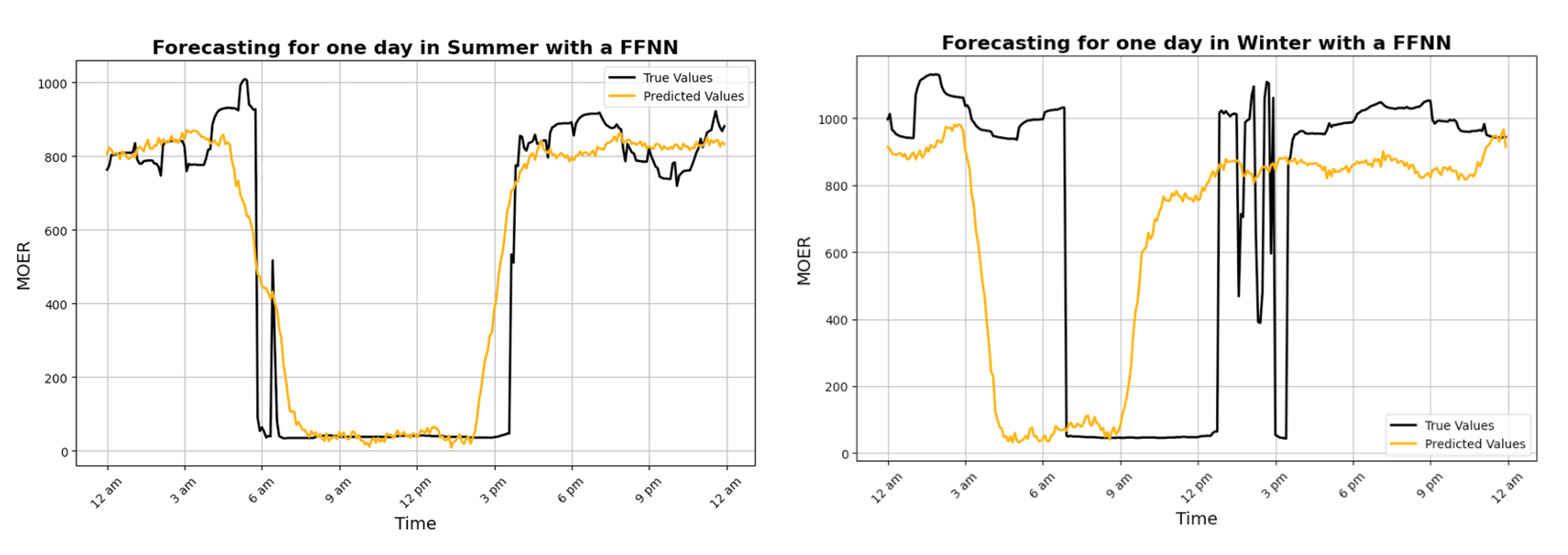
Summer Huber loss = 77.8 (consistent solar pattern) and Winter Huber loss = 320.6 (spike timing error ±4 hours)
FFNN treats each 1000-point window independently, but winter weather evolves sequentially (cloud system persists 2-3 days for instance). We need a model with a temporal memory.
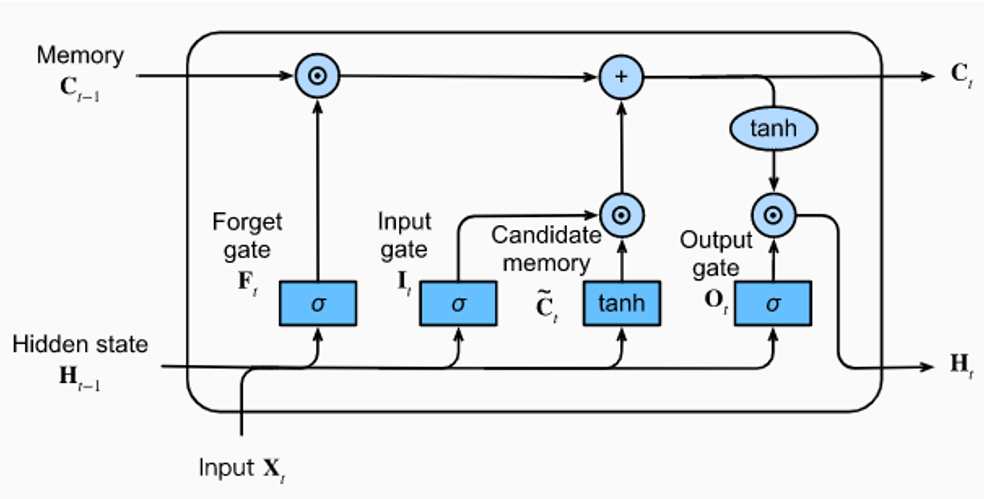
Long Short-Term Memory (LSTM)
Recurrent architecture maintains hidden state across timesteps, capturing sequential dependencies. A typical LSTM architecture is composed of 4 FFNN (3 gates, 1 candidate) and process the cell state and hidden state (long and short-term memories) from the previous LSTM cell:
- Training data: 25 days to predict 1 full day
- Window size: 20 timesteps (100 minutes)
- Epochs: 10 (convergence validated on held-out validation set)
- Preprocessing: DART library scaling + day/month co-variates
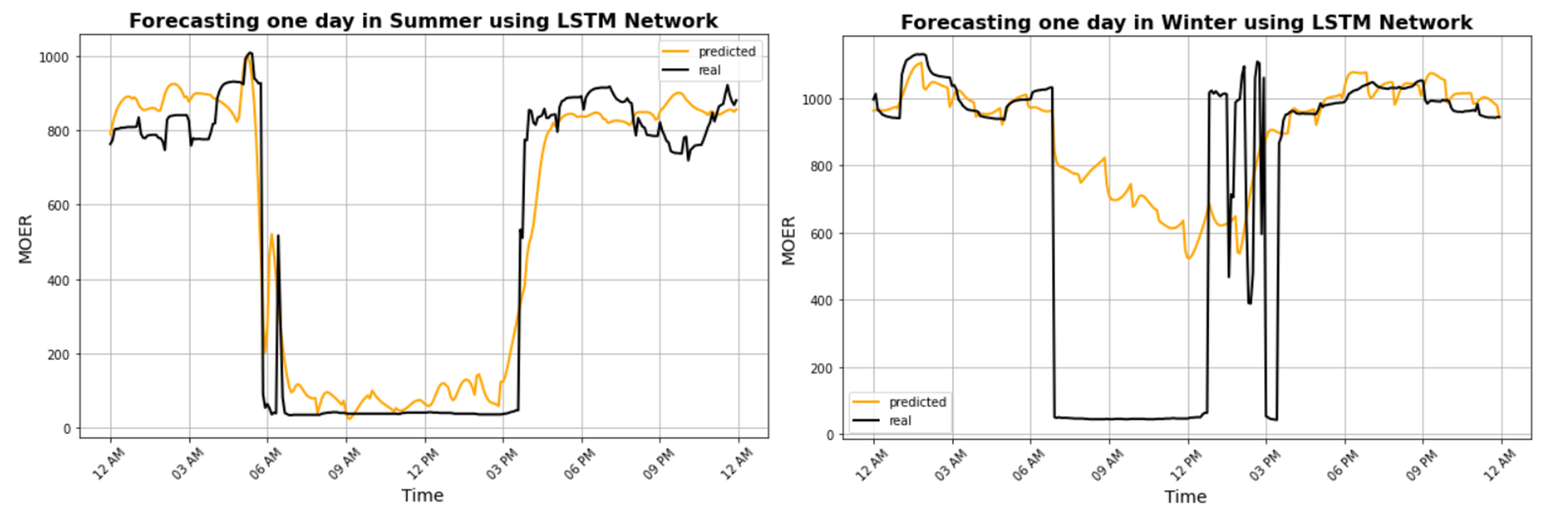
Summer: Huber loss = 78.6 (same as FFNN) and Winter: Huber loss = 231.9 (28% improvement, spike timing ±30 min)
Model Comparison
| Season | FFNN Huber Loss | LSTM Huber Loss | Spike Timing Error |
|---|---|---|---|
| Summer | 77.8 | 78.6 | <15 min (both) |
| Winter | 320.6 | 231.9 | FFNN ±4h / LSTM ±30min |
LSTM better captures when spikes occur even if magnitude is 2-3× off.
5- Battery Modeling
Battery terminal voltage is non-linear with SOC and differs between charging/discharging due to electrochemistry:
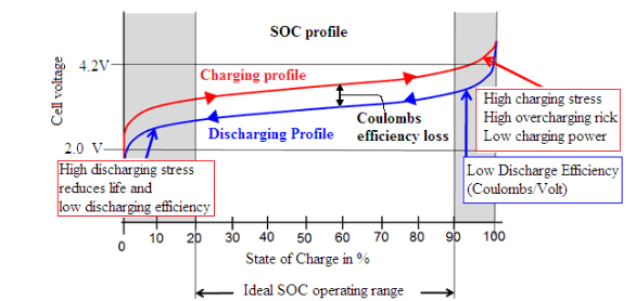
We generate high-granularity charging/discharging curves across 0-100% SOC to derive convex power-SOC relationships.
Charging Power Limit
Battery voltage rises slowly 0-95% SOC (constant current), then rapidly 95-100% (constant voltage taper). Two-piece convex model:
$$ P_{\text{charge}}(SOC) = \begin{cases} 142.8 \log(SOC) + 8755.4 & \text{for } SOC \in [0, 0.95] \\ -175107.3 \cdot SOC + 175107.3 & \text{for } SOC \in (0.95, 1] \end{cases} $$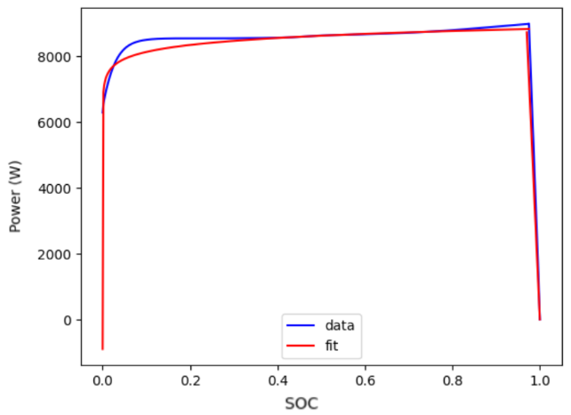
Discharging Power Limit
$$ P_{\text{discharge}}(SOC) = 306.3 \log(SOC) + 8838.8 $$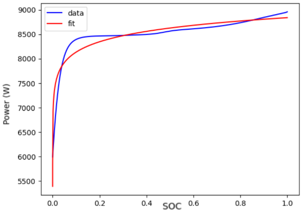
6- Optimization
Three charging strategies are compared across 6,844 real residential sessions:
- Baseline: Plug in → charge to 100% → stop
- Shift Charging: Charge opportunistically during low-emission windows → reach target SOC
- Vehicle-to-Grid (V2G): Discharge during high-emission peaks + charge during clean windows
Objective: Minimize total emissions over the charging session
$$ \min_{P(t), I(t), SOC(t)} \sum_{t=0}^{T} \text{MOER}(t) \times P(t) \times \Delta t $$where MOER(t) is the forecasted emission curve, P(t) charging power, Δt = 5 min.
Constraints
SOC dynamics (state equation): $$ SOC(t+1) = SOC(t) + \frac{I(t)}{Q} \Delta t $$
Power-current relationship (resistive losses): $$ P(t) \geq V \cdot I(t) + C \cdot |I(t)| $$
Power limits (battery physics + charger rating): $$ \begin{cases} 0 \leq P(t) \leq \min(P_{\text{charge}}(SOC), P_{\text{limit}}) & \text{(shift charging)} \\ P_{\text{discharge}}(SOC) \leq P(t) \leq P_{\text{charge}}(SOC) & \text{(V2G)} \end{cases} $$
Boundary conditions (from charging session data): $$ \begin{align*} SOC(t=0) &= SOC_{\text{start}} \quad \text{(initial SOC from previous trip)} \\ SOC(t=T) &\geq SOC_{\text{target}} \quad \text{(required SOC for next trip)} \end{align*} $$
Parameters
| Symbol | Description | Value |
|---|---|---|
| $P_{\text{charge}}(SOC)$ | Max charging power | From battery model |
| $P_{\text{discharge}}(SOC)$ | Max discharging power | From battery model |
| $P_{\text{limit}}$ | Charger power rating | 9.6 kW (Level 2: 240V × 40A) |
| $V$ | Charging voltage | 240 V |
| $Q$ | Pack capacity | 250 Ah |
| $C$ | Loss coefficient | 36 (~15% round-trip efficiency) |
| $\Delta t$ | Time resolution | 5 min |
| $SOC_{\text{start}}, SOC_{\text{target}}$ | Initial/final SOC | From charging data |
This optimization problem is solved using CVXPY.
7- Results & Discussion
Results
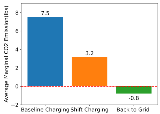
| Strategy | Avg CO2 (lbs) | Reduction vs Baseline |
|---|---|---|
| Baseline | 7.5 | — |
| Shift Charging | 3.2 | -57% |
| Vehicle-to-Grid | -0.8 | -111% (net negative) |
The net-negative V2G result stems from avoided emissions, which are recorded as negative in the carbon balance.
Limitations
- LSTM winter predictions: Huber Loss >100, accurately predicts spike timing but struggles with magnitude
- Simplified battery model: Limited variables, logarithmic SOC relationship only, excludes temperature and aging effects
- Geographic mismatch: Norway charging data substituted for unavailable California data so numerical CO2 values are theoretical, though the framework is conceptually valid
Next Steps
- Explore additional variables to improve emission prediction accuracy
- Incorporate battery temperature and electrochemistry parameters for more accurate power limits
- Explore additional scenarios: electricity price curves, battery protection from low SOC
Python · PyTorch · Darts · LSTM · CVXPY · PyBamm · pandas · numpy · matplotlib · WattTime API