1- Overview
Note: This is a personal review and reminder of the image-to-image translation concepts and architectures explored during my time at the French National Gendarmerie, illustrated with a small application on the CUHK face-sketch dataset.
Sketch-to-Face Translation - Concepts & Architectures
2- Context & Motivation
Problem Statement
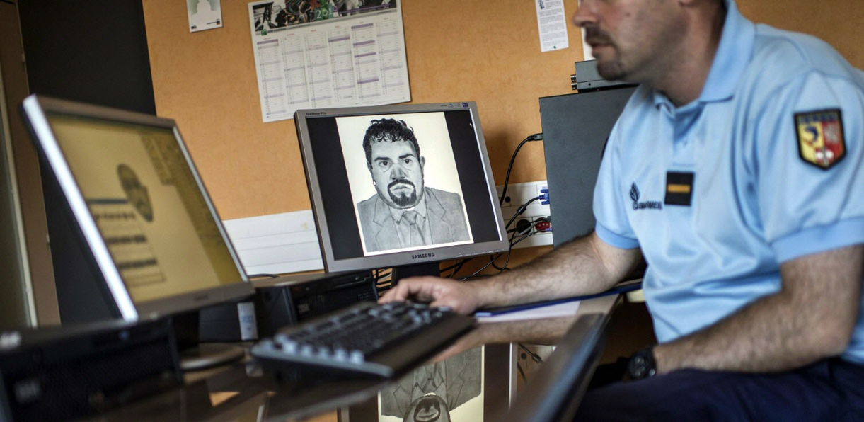
Forensic facial composites are the primary tool investigators use when no photograph of a suspect is available. Produced from witness descriptions, they are sketch-like pictures that capture facial geometry but lose everything about texture, color, skin, lighting, and photographic realism. The challenge is to generate all that missing information in a way that is simultaneously:
- Structurally faithful: the generated face must match the sketch’s geometry
- Photorealistic: it must look like an actual photograph, not a cartoon or a blur
- Generalisable: it must work on sketches it has never seen before
This is an image-to-image translation problem: the model must learn a complex mapping from one visual domain (sketches) to another (photographs), with no intermediate supervision on what the missing texture should look like.
Goal of this page
Explore sketch-to-photo face generation algorithms, progressing from a simple autoencoder baseline to a full conditional GAN (Pix2Pix).
3- Core concepts
Convolutional Neural Network (CNN)
For images, convolutional layers apply a small filter that slides across the image and detects local patterns (edges, then shapes, then high-level features). This is far more efficient than connecting every pixel to every neuron.
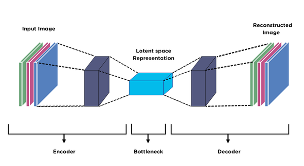
Encoder
An encoder is a CNN that progressively downsamples the image, compressing it into a compact bottleneck vector. Spatial resolution decreases while the number of abstract feature channels increases.
Decoder
It is the mirror of the encoder. It takes the compressed bottleneck and progressively upsamples it back to the original resolution using transposed convolutions.
Autoencoder = Encoder + Decoder
For image translation, we feed a sketch as input and train the decoder to output a photo. The network learns to translate domains through the bottleneck. However, fine spatial details (exact eye shape, hair positions) are lost in compression and hard to recover. This is the fundamental limitation of the pure autoencoder.
U-Net
The U-Net (Ronneberger et al., 2015) adds direct shortcuts that copy feature maps from each encoder layer to the corresponding decoder layer. The decoder can then use both high-level semantic context (from the bottleneck) and low-level spatial details (from the skip connections), producing sharper, more faithful outputs.
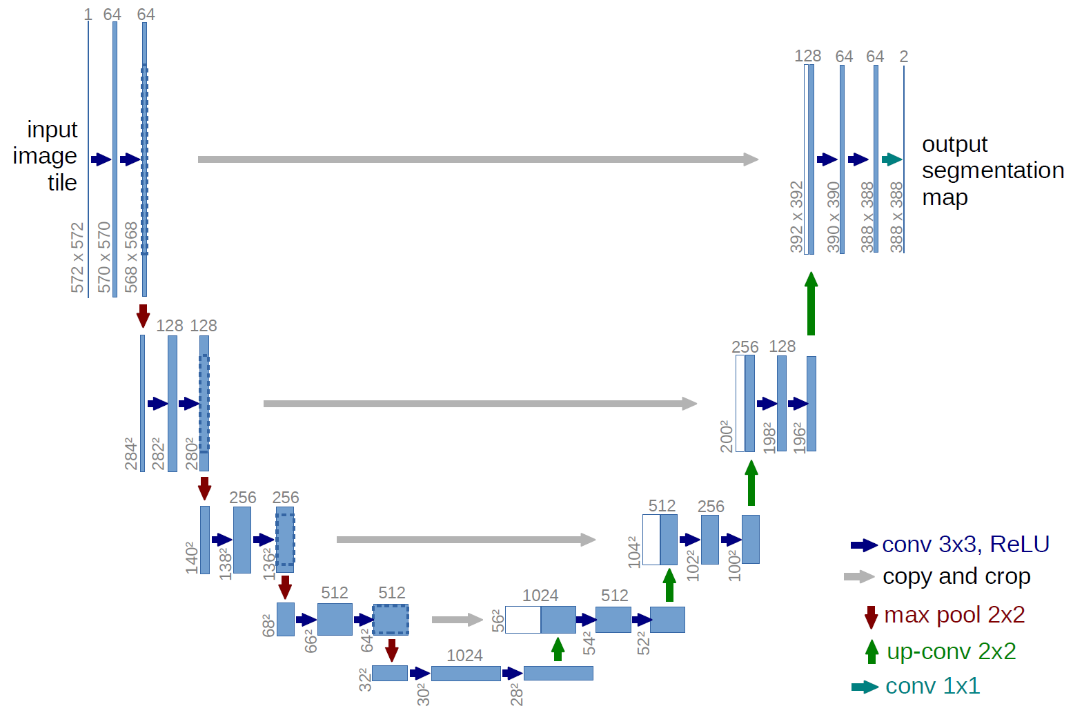
Skip connections allow the decoder to receive both the abstract semantic representation from the bottleneck and the precise spatial information preserved from early encoder layers.
GAN (Generative Adversarial Network)
Even with U-Net, training with MAE loss tends to produce blurry outputs. Indeed, MAE loss averages over all plausible outputs so if the network is uncertain between two plausible textures, it averages them, producing blur. A GAN solves this by adding a second network, the discriminator, trained adversarially against the generator:
$$\mathcal{L}_{\text{GAN}} = \mathbb{E}[\log D(x, y)] + \mathbb{E}[\log(1 - D(x, G(x)))]$$
where $x$ is the sketch (condition), $y$ is the real photo, $G(x)$ is the generated photo. The adversarial loss landscape forces G to produce sharp, realistic details, because any blurriness is immediately detected by D as fake.
Pix2Pix
Pix2Pix (Isola et al., 2017) combines U-Net + PatchGAN for paired image-to-image translation. The PatchGAN discriminator classifies 70×70 overlapping patches as real/fake rather than the whole image, hence forcing local texture realism everywhere, not just global plausibility.
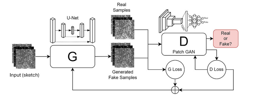
The MAE term anchors the output structurally close to the real photo while the GAN term forces local realism on top.
4- Example of potential application on the CUHK dataset
CUHK Face Sketch Database
This the standard academic benchmark for face sketch-to-photo synthesis. It contains paired sketch/photo examples drawn by art students from real photographs.
| Split | Pairs |
|---|---|
| Training | ~550 |
| Test | ~56 |
The dataset is very small by deep learning standards. To increase diversity and reduce overfitting, data augmentation is applied on-the-fly (flips and rotations, symmetrically to sketch/photo pairs to preserve pairing consistency).
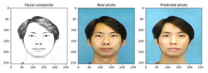
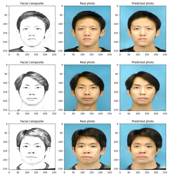
Results
Three examples from the test set: facial composite → real photo → model prediction:
Evaluation metrics: SSIM and PSNR
Visual inspection is the natural first approach for this type of task, but it does not allow reproducible model comparison. Two metrics are standard for generated image quality.
PSNR (Peak Signal-to-Noise Ratio) measures the ratio between the maximum possible pixel value and the power of the reconstruction noise, expressed in decibels:
$$\text{PSNR} = 10 \cdot \log_{10}\left(\frac{\text{MAX}^2}{\text{MSE}}\right) \qquad \text{avec} \quad \text{MSE} = \frac{1}{N}\sum_{i=1}^{N}(y_i - \hat{y}_i)^2$$
where MAX is the maximum pixel value (255 for an 8-bit image), and MSE is the mean squared error between the real image $y$ and the generated image $\hat{y}$. Higher PSNR means more faithful reconstruction. PSNR > 20 dB is generally considered acceptable for face synthesis.
SSIM (Structural Similarity Index) evaluates the perceptual similarity between two images by combining three components: luminance, contrast and structure:
$$\text{SSIM}(y, \hat{y}) = \frac{(2\mu_y\mu_{\hat{y}} + c_1)(2\sigma_{y\hat{y}} + c_2)}{(\mu_y^2 + \mu_{\hat{y}}^2 + c_1)(\sigma_y^2 + \sigma_{\hat{y}}^2 + c_2)}$$
where $\mu$ denotes the local mean, $\sigma^2$ the local variance, $\sigma_{y\hat{y}}$ the cross-covariance, and $c1, c2$ stabilization constants. SSIM ranges in $[−1,1]$, with 1 indicating perfect similarity. Unlike PSNR, it is designed to better reflect human perception of image quality.
On the example above, SSIM≈0.64 and PSNR≈19.3 dB, limited by available computer performance. For Pix2Pix applied to the same dataset, reported reference values are SSIM≈0.70 and PSNR≈18.4 dB in baseline configuration, improving to SSIM≈0.81 and PSNR≈23.0 dB with sketch gamma inversion preprocessing. These values are consistent with mine. Results depend on training duration, data quantity and augmentation, and available hardware.
Python · TensorFlow / Keras · NumPy · Matplotlib · PIL