1- Overview
A large-scale research study analyzing 2.4M+ California mobile phone users’ mobility patterns to inform the state’s 2030 greenhouse gas reduction policy - combining machine learning, geospatial big data analysis, and network science.
2- Context & Motivation
Problem Statement
California has committed to reducing greenhouse gas emissions 40% below 1990 levels by 2030. Transportation is the single largest contributor to those emissions, and Vehicle Miles Traveled (VMT) is the primary lever. The COVID-19 pandemic created an unprecedented natural experiment: a sudden, statewide disruption to mobility that revealed which travel behaviors are habitual (and reversible) and which are structural (and permanent).
The California Air Resources Board (CARB), in partnership with UC Berkeley and Lawrence Berkeley National Laboratory, commissioned this study to quantify those shifts and translate them into actionable policy guidance.
Technical challenge
Understanding mobility at this scale requires solving three distinct problems simultaneously: inferring travel mode (car vs. walking) from raw GPS pings without any labeled training data, detecting residential relocations from nighttime location patterns, and measuring network-level changes in commute structure across ~8,000 census tracts over four years. Each requires a different algorithmic approach — unsupervised, semi-supervised, and graph-theoretic respectively.
Project goal
Measure COVID-19’s impact on VMT, commute patterns, and residential relocation across California at census-tract granularity using four years of anonymized LBS data, and derive targeted VMT reduction strategies by region and demographic group to inform CARB’s 2030 climate roadmap.
3- Dataset
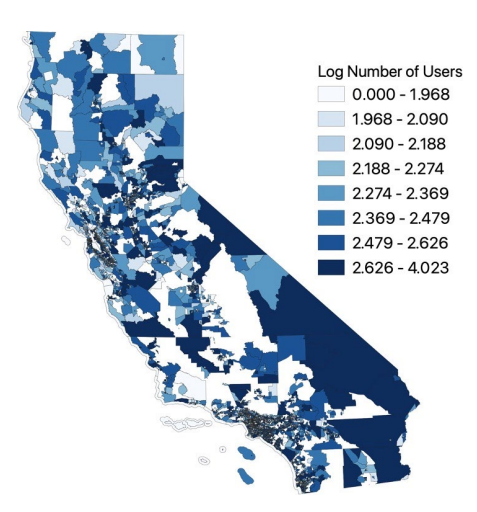
Location-Based Service (LBS) data sourced from Spectus: anonymized mobile phone GPS pings collected across California from 2019 to 2022.
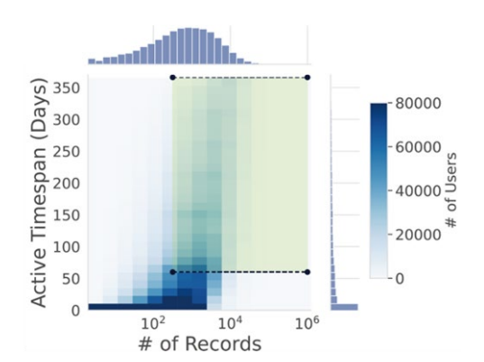
Spatial resolution: Census block group (~600–3,000 people). Quality filters applied to retain only users with sufficient coverage: >316 pings, >60 active days.
Home and work location detection uses a heuristic based on the most frequently visited location during the appropriate time window:
home = most_freq_location(user, time_range="7pm-7am", min_visits=10)
work = most_freq_location(user, time_range="7am-7pm", weekdays_only=True, min_visits=10)
Final Dataset:
| Year | Total users | High-quality users | Users with Home and Work Found |
|---|---|---|---|
| 2019 | 9.4M | 3,482,574 | 861,167 |
| 2020 | 5.9M | 2,396,990 | 431,190 |
| 2021 | 5.2M | 2,036,110 | 465,311 |
| 2022 | 5.6M | 2,582,405 | 702,847 |
4- Methodology
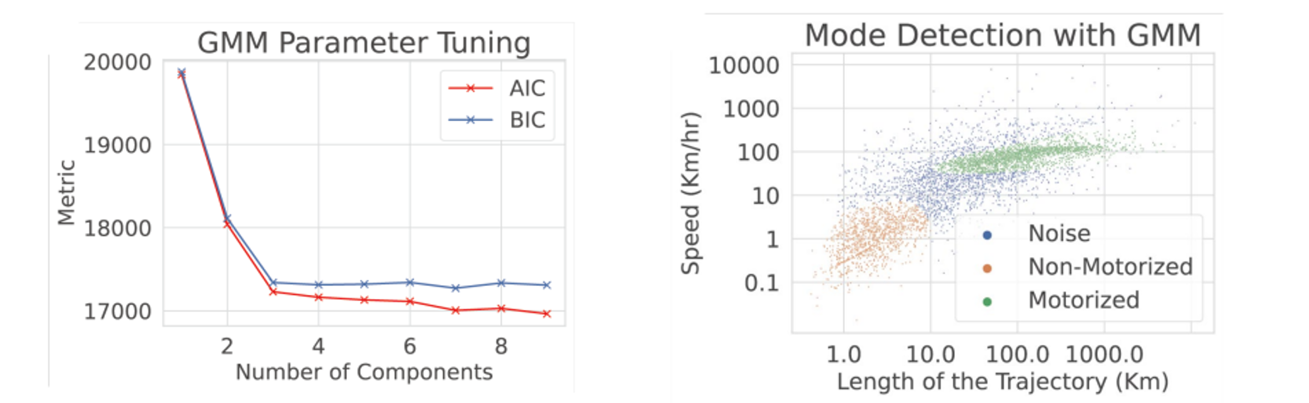
Algorithm 1 - Mode Detection via GMM
No labeled trip data is available so we cannot train a supervised classifier because we do not know the ground truth mode for any trip. We need to infer travel mode purely from the structure of the data itself. Two signals suffice to separate motorized from non-motorized trips: how fast the trip went, and what distance it covered. A car trip and a walking trip occupy very different regions in (speed, distance) space. Even without labels, these clusters should be visible.
A Gaussian Mixture Model (GMM) assumes the data was generated by a mixture of $k$ Gaussian distributions, each representing a natural cluster. Rather than assigning each point to one cluster like K-Means clustering, a GMM produces a probability of belonging to each cluster. This matters here because some trips are genuinely ambiguous (a slow car ride looks like a fast bike ride in this feature space).
Formally, the probability of observing a feature vector $X$ is:
$$\text{GMM}(X) = \sum_{k=1}^{3} \pi_k ,\mathcal{N}(X \mid \mu_k, \Sigma_k)$$
where $\pi_k$ is the weight of component $k$, $\mu_k$ its mean, and $\Sigma_k$ its covariance. The model is fitted by Expectation-Maximization: alternate between assigning probabilities to each point given current parameters, and updating parameters given current assignments.
We use the AIC/BIC elbow method to determine the number of clusters k. Both measure model fit penalized by complexity:
$$\text{AIC} = 2p - 2\ln(\hat{L}) \qquad \text{BIC} = p\ln(n) - 2\ln(\hat{L})$$
where $p$ is the number of parameters, $n$ the number of observations, and $\hat{L}$ the maximized likelihood. Plotting AIC/BIC against $k$ produces an “elbow”. This is the point where adding more components stops improving the score meaningfully. Here that elbow falls at $k=3$, confirming three natural clusters.
Radius of Gyration
The radius of gyration $r_g$ is a single number summarizing how spatially dispersed a user’s movements are. It is the typical radius of a person’s daily activity bubble. It borrows from physics, where the radius of gyration of a mass distribution measures how spread out the mass is around its center.
$$r_g(u) = \sqrt{\frac{1}{n_u} \sum_{i=1}^{n_u} \text{dist}\left(r_i(u),\ r_{cm}(u)\right)^2}$$
where $r_i(u)$ are all visited locations and $r_{cm}(u)$ is their weighted centroid (center of mass). It is essentially the root-mean-square distance from home. High $r_g$ signals car-dependent, long-distance travel, typical of rural residents. Low $r_g$ signals compact, walkable mobility, typical of urban residents.
By tracking $r_g$ before and after lockdown, we quantify not just whether people traveled less, but whether they traveled shorter distances, a distinction that matters for VMT policy.
Algorithm 2 - Home Change Detection via KMeans-SVM
The challenge is to detect intra-state residential moves (>=5 miles) from nighttime GPS patterns, without any labeled relocation data. Distinguishing a genuine move from noisy patterns (vacation, travel, temporary stay) requires a robust boundary.
K-Means (unsupervised) partitions nighttime locations into 2 clusters by minimizing within-cluster variance:
$$\underset{C_1, C_2}{\arg\min} \sum_{k=1}^{2} \sum_{x_i \in C_k} | x_i - \mu_k |^2$$
Applied to (latitude, longitude, days since Jan 1), the two clusters naturally represent “nights before the move” and “nights after the move”, giving pseudo-labels for the next step.
Support Vector Machine (SVM) with wide margin (supervised) finds the hyperplane that maximizes the margin between the two classes. Using $C = 0.01$ forces a very wide margin. The classifier prefers to misclassify a few ambiguous nights rather than draw a tight boundary that overfits to geographic noise. This prevents treating a week-long vacation as a move.
The move date is estimated as the boundary between the two clusters:
$$\text{MoveDate} = \min\bigl(\max(C_{\text{before}}),\ \max(C_{\text{after}})\bigr)$$
Algorithm 3 - Louvain Community Detection
From GPS pings to a network: Rather than analyzing individual trips, we build a graph of the aggregate commute structure of California. Each census tract is a node, an edge connects two tracts if users commute between them, weighted by the number of such commuters. This gives a directed weighted graph of ~8,000 nodes and up to 145,000 edges.
Louvain community detection algorithm identifies groups of nodes that are more densely connected internally than to the rest of the network, natural commute catchment areas. It does this by maximizing modularity $Q$, which measures how much more within-community flow exists compared to what would be expected by chance:
$$Q = \frac{1}{2m} \sum_{i,j} \left[ A_{ij} - \frac{k_i k_j}{2m} \right] \delta(c_i, c_j)$$
where $A_{ij}$ is the edge weight between tracts $i$ and $j$, $k_i$ the total weight of edges touching node $i$, $m$ the sum of all edge weights, and $\delta(c_i, c_j) = 1$ if $i$ and $j$ belong to the same community.
High $Q$ means strong regional isolation, commuters stay within their catchment area. Low $Q$ means an integrated network where people freely cross regional boundaries. Tracking $Q$ and the number of communities year-over-year reveals whether COVID permanently fragmented California’s commute geography.
5- Results
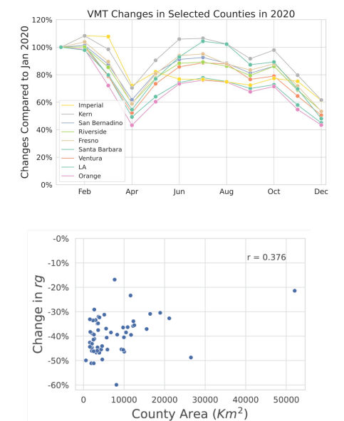
VMT reduction & regional disparities
Urban counties (LA, Orange, Santa Barbara) saw 38–55% VMT reductions in April 2020, rural counties (Imperial, Kern) only 20–30%. The 20-percentage-point gap reflects fundamentally different vehicle dependency: urban residents could substitute car trips for walking or remote work, rural residents largely could not. A positive correlation (r=0.376) between county area and VMT persistence confirms this vehicle dependency is structural, not behavioral.
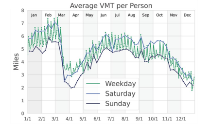
COVID-19 did not change the within-the-week variation in VMT, the weekly patterns are preserved. At the beginning of the lockdown, we observe a larger reduction in VMT on weekends compared to weekdays.
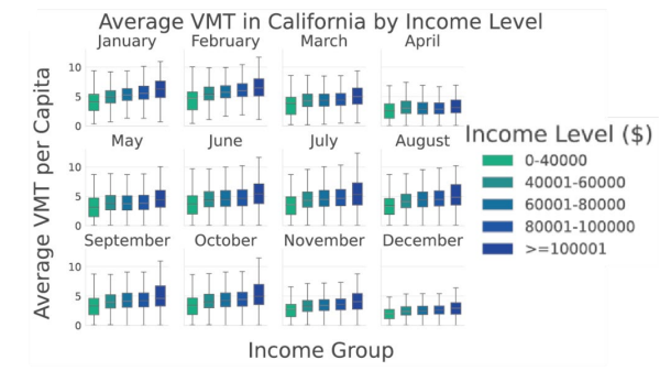
No notable differences across different income groups in VMT reduction. Tracts with higher median income showed a faster VMT rebound, likely reflecting greater flexibility for remote work.
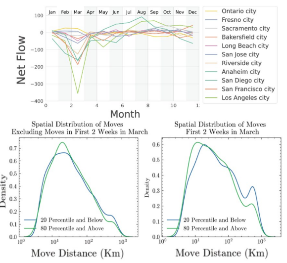
Residential relocation
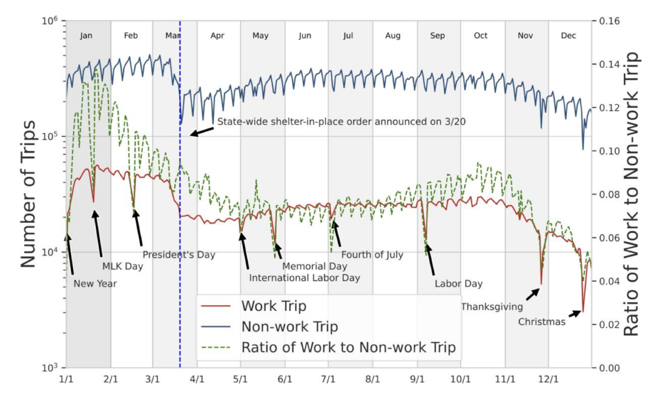
A sharp spike in moves occurred in the 15-day window between the State of Emergency (March 4) and the Shelter-in-Place order (March 19, 2020).
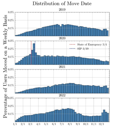
The distance distribution during this crisis window was bimodal: one mode at ~50 miles (local reshuffling within metro areas) and one at ~350 miles (inter-regional). We observe more moves over longer distance in the 2-week period, and large urban areas experience large net outflow. Immigration and emigration in cities in the Central Valley such as Bakersfield and Fresno remain stable.
Trip purpose & commute network fragmentation
Non-commute travel (shopping, leisure) recovered to near-baseline levels by 2022. Commute trips did not — the work-to-non-work ratio never returned to its pre-pandemic level. Remote and hybrid work restructured not just where people work, but the fundamental shape of California’s daily travel demand.
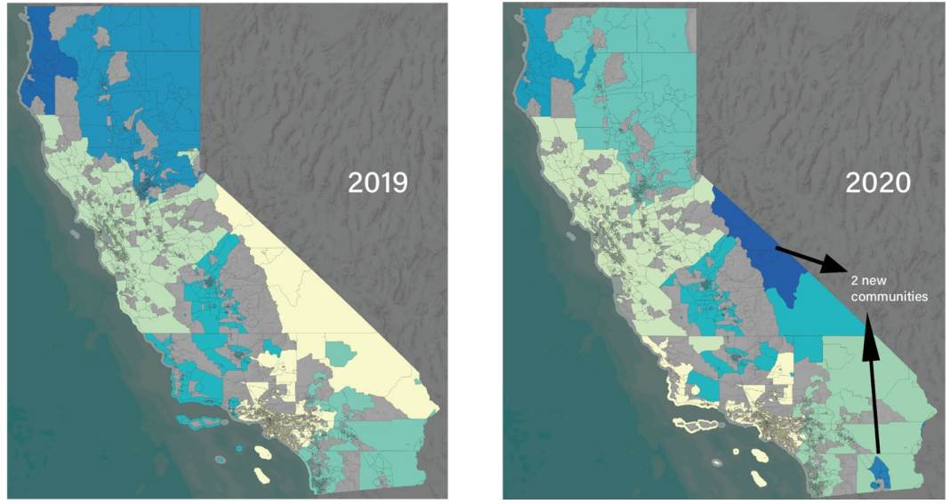
| Year | Edges | Communities | Modularity |
|---|---|---|---|
| 2019 | 145,838 | 6 | 0.628 |
| 2020 | 89,382 | 8 | 0.653 |
| 2021 | 73,401 | 8 | 0.648 |
| 2022 | 111,652 | 8 | 0.666 |
The network lost 38.7% of its edges in 2020. Two new isolated communities emerged in remote regions (El Centro, eastern Sierras). Crucially, modularity remained elevated through 2022. Even as some edges recovered, the network never returned to its pre-pandemic integrated structure. Major urban centers (SF, LA, San Diego) continue to act as commute gravity wells over their surrounding regions.
6. Impact & Policy Recommendations
Validated outcomes: LBS data confirmed as a viable, cost-effective alternative to expensive travel surveys. Reusable open-source algorithms for mode detection and relocation analysis without labeled training data have been developed and CARB 2030 roadmap informed with census-tract-level VMT reduction targets. The results translate into four concrete policy levers for CARB’s 2030 strategy:
Urban areas can leverage the structural reduction in vehicle dependency post-COVID: zoning reforms near transit, reduced parking minimums, and suburban infill development would lock in these gains rather than allowing car use to creep back.
Rural areas present the harder problem: vehicle dependency persisted precisely where alternatives are absent. EV charging infrastructure and carpool lanes address the emissions dimension without requiring behavioral change.
Remote work is now structurally embedded in California’s labor market. Land use policy should adapt by encouraging residential development near suburban employment centers and reducing commute-driven VMT.
Micro-mobility at scale is the only intervention category shown to move the needle on modal shift. Policy should prioritize rapid deployment density over geographic coverage breadth.
Python · pandas · numpy · scikit-learn · networkx · geopandas · matplotlib