1- Overview
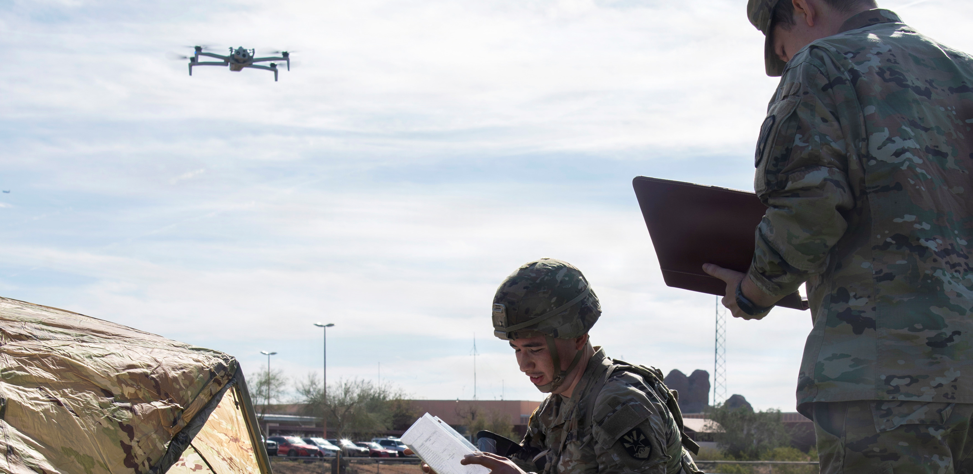
An end-to-end computer vision system for aerial imagery, implemented and validated on a commercial drone for real-time video inference & counter UAS interceptor simulation
2- VisDrone Dataset
Understanding VisDrone
VisDrone is the standard benchmark for drone-based object detection, created by Tianjin University for international computer vision competitions. The dataset represents real-world drone footage captured at various altitudes (20-500 meters), angles, and lighting conditions across Chinese cities.
The dataset contains 6,471 training images and 548 validation images across 10 object classes: pedestrian, car, van, truck, bus, bicycle, motor, tricycle, awning-tricycle, and people. Each image is densely annotated with bounding boxes, occlusion flags, and truncation indicators.
The Small Object Challenge
To understand why aerial detection is hard, consider the object size distribution. In standard benchmarks like COCO (Common Objects in Context, one of the most widely used benchmark datasets in computer vision), a person typically occupies 200×400 pixels and a car occupies at least 150×80 pixels. In VisDrone, 67% of annotated objects have an area smaller than 1,000 pixels squared, equivalent to a 30×30 square. The median object size is just 340 pixels squared, approximately 18×18 pixels.
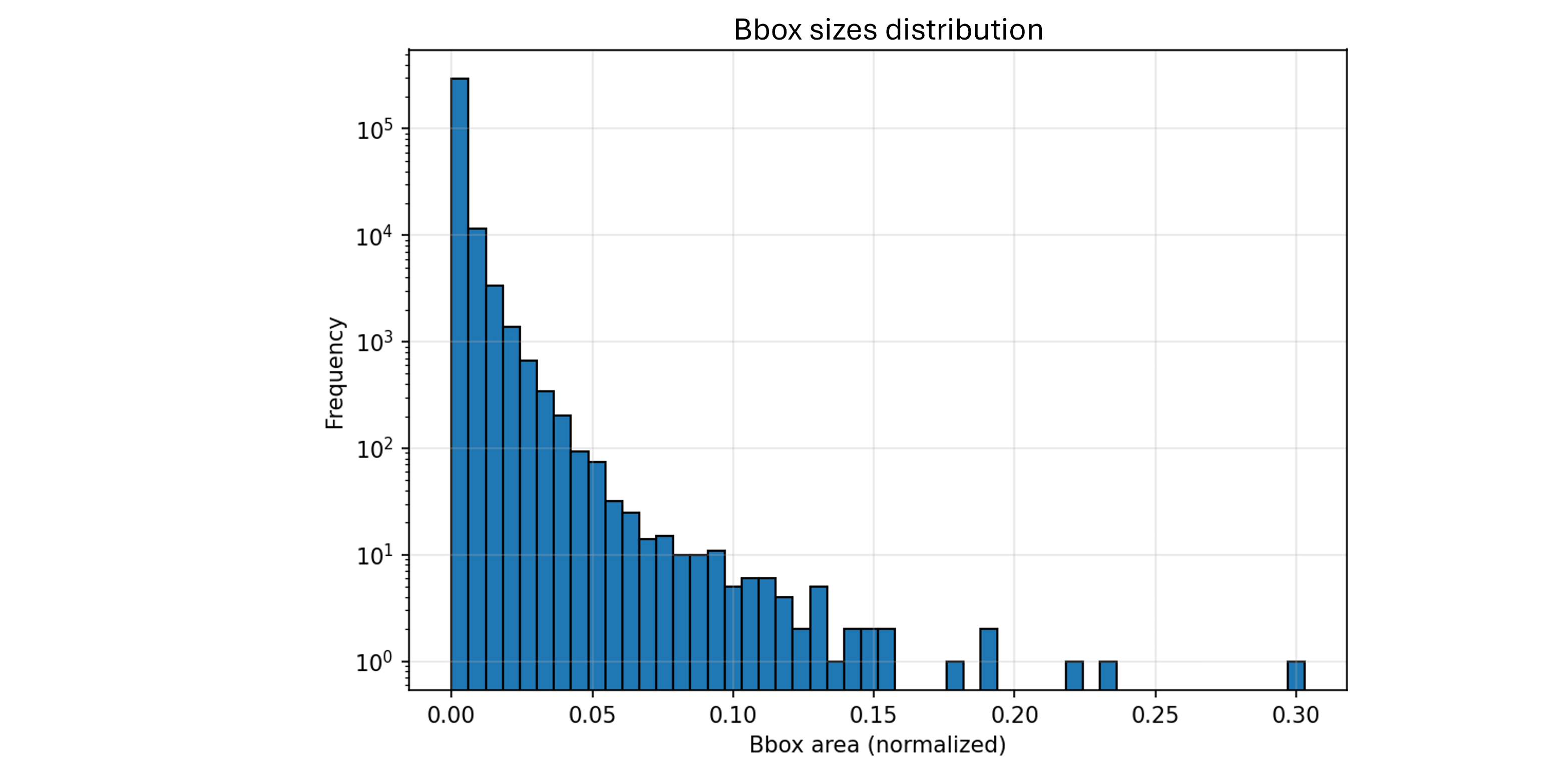
This isn’t a minor difference but a fundamentally different problem. When a pedestrian is represented by an 8×6 pixel box, traditional feature extractors struggle because there simply aren’t enough pixels to encode distinguishing characteristics. The network must learn to extract signal from extremely sparse visual information.
Class Imbalance and Scene Density
The dataset exhibits severe class imbalance. Cars represent 144,867 instances (46% of all annotations), while bicycles account for only 10,480 instances (3.3%). More problematically, two classes (people and awning-tricycle) appear in the validation set but not in training, creating a zero-shot detection scenario for these categories.
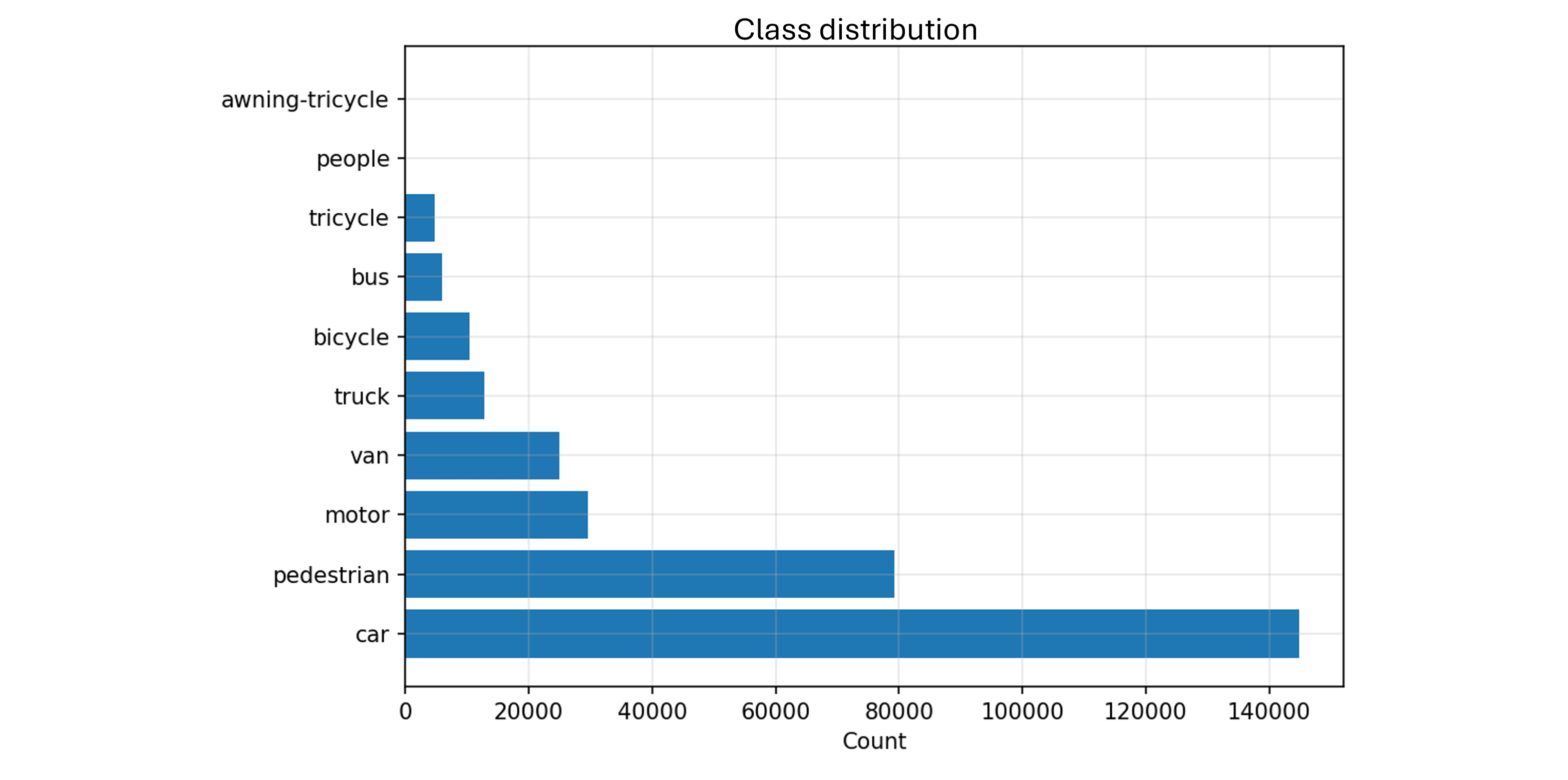
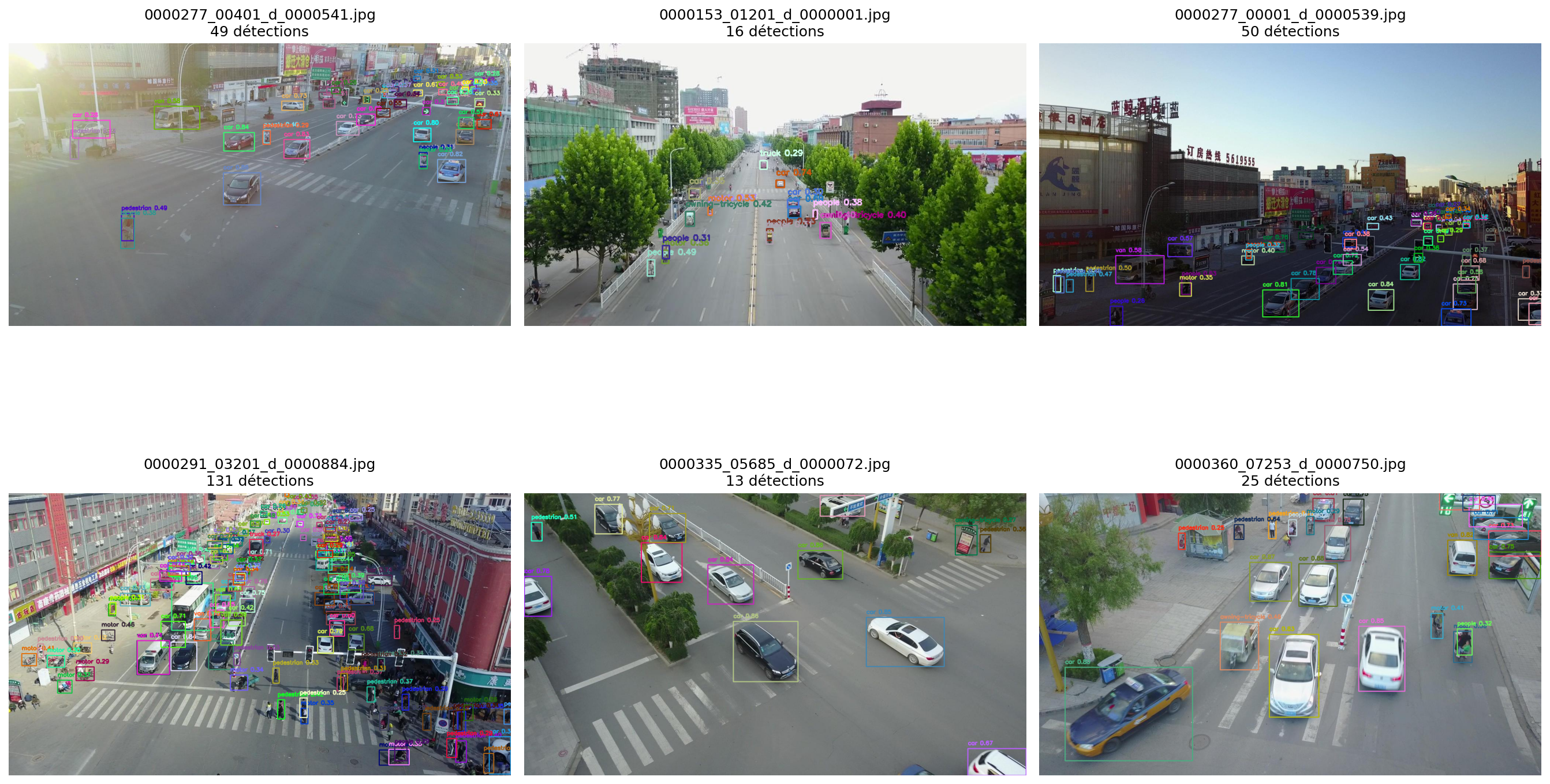
Beyond individual object difficulty, scenes are exceptionally dense. Images contain an average of 48 objects, with some frames exceeding 130 instances. This creates significant occlusion where objects overlap, particularly in traffic scenarios where vehicles cluster at intersections.
3- YOLO Model Training
The Detection Problem Formulation
Object detection requires solving two tasks simultaneously: classification (what is this object?) and localization (where exactly is it?). The field divides into two architectural approaches.
Two-stage detectors like Faster R-CNN first generate region proposals through a Region Proposal Network, then classify each proposal. This separation allows high accuracy but at the cost of speed, typically achieving 5-10 FPS on CPU.
One-stage detectors like YOLO treat detection as a regression problem, predicting bounding boxes and class probabilities directly in a single forward pass. This enables real-time inference at 20-30 FPS on CPU, critical for live drone applications.
For this project, YOLOv8 was selected specifically for its combination of speed, anchor-free design, and multi-scale detection capabilities.
YOLOv8 Architecture Deep Dive
YOLOv8 consists of three main components: a backbone for feature extraction, a neck for multi-scale feature fusion, and a head for final predictions.
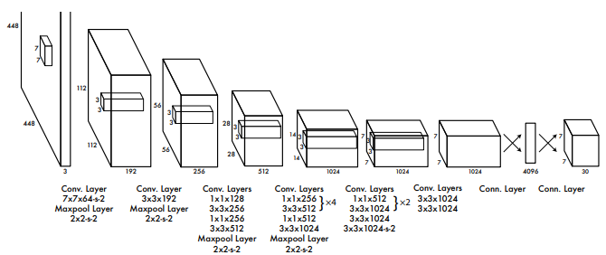
Backbone (CSPDarknet)
The backbone extracts hierarchical features through a series of convolutional layers. Early layers detect low-level patterns like edges and textures. Middle layers identify object parts such as wheels, windows, or human limbs. Deep layers encode high-level semantic information about complete objects.
The Cross Stage Partial (CSP) structure splits the feature map into two parallel paths, allowing gradients to flow through different routes. This improves learning efficiency while reducing computational cost, critical for maintaining real-time performance.
Neck (PANet Feature Pyramid)
The neck implements a Path Aggregation Network to fuse features across different scales. This addresses a fundamental challenge in aerial detection: the same image contains both very small objects (distant pedestrians at 10×10 pixels) and large objects (nearby buses at 100×60 pixels).
The Feature Pyramid Network creates multiple detection heads at different resolutions. High-resolution feature maps preserve spatial detail for small objects. Low-resolution feature maps provide semantic context for large objects. PANet adds bottom-up path augmentation, allowing fine-grained localization information from high-resolution features to reach all prediction layers.
Detection Head (Anchor-Free)
Unlike previous YOLO versions that used predefined anchor boxes, YOLOv8 employs an anchor-free approach. For each spatial location, the network directly predicts the distance to the four bounding box edges (left, top, right, bottom) and the object class probabilities.
The anchor-free design is particularly advantageous for aerial imagery where object aspect ratios vary unpredictably. A car seen from directly above is nearly square, while a car at an oblique angle becomes elongated. Predefined anchors would need to cover all these variations, increasing model complexity.
Loss Function: Training Objectives
YOLOv8 optimizes a composite loss function with three components:
Classification Loss
Binary cross-entropy measures how well the network identifies object classes. For each predicted box, the model outputs a probability distribution over the 10 classes. The loss penalizes deviations from the true class label.
Box Regression Loss
Complete IoU (CIoU) loss quantifies localization accuracy. Unlike simple L2 distance between coordinates, CIoU considers the overlap ratio, center point distance, and aspect ratio difference between predicted and ground truth boxes. This produces tighter, more accurate bounding boxes.
Distribution Focal Loss
To handle class imbalance (cars vastly outnumber bicycles), the model applies focal loss which down-weights easy examples and focuses learning on hard examples. This prevents the dominant car class from overwhelming gradient updates and ensures the model learns to detect rare classes.
Why YOLOv8n Specifically
The YOLOv8 family includes five variants (n, s, m, l, x) trading accuracy for speed. YOLOv8n (nano) was chosen for this project, enabling CPU inference at acceptable framerates. Larger variants would achieve higher mAP but cannot run in real-time on consumer hardware, which defeats the purpose for live drone applications.
Data Augmentation for Small Objects
Standard augmentation techniques (random flips, brightness adjustments) are insufficient for tiny objects. Random cropping, for instance, risks completely removing a 20×20 pixel object from the frame.
Mosaic Augmentation
The most impactful technique combines four random images into a single training sample. Each batch effectively sees 4× more object instances with diverse contexts and scales. This simulates altitude variation within a single image and forces the model to handle objects at different relative sizes simultaneously.
Multi-Scale Training
Images are randomly resized between 0.5× and 1.5× their original dimensions during training. This creates synthetic altitude variations and ensures the model generalizes across different flight heights without needing altitude-specific datasets.
HSV Color Jittering
Hue, saturation, and value are randomly perturbed to simulate different lighting conditions, times of day, and weather. This is critical for deployment robustness when the drone operates in varied environments.
Training Configuration
The model was trained on Google Colab with a Tesla T4 GPU (16GB VRAM) for 35 epochs with batch size 32. The Adam optimizer was used with an initial learning rate of 0.01, decaying by cosine annealing. Total training time was approximately 1.5 hours.
Data was split 92% training (6,471 images) and 8% validation (548 images). The validation set was held completely separate and never seen during gradient updates, providing an unbiased estimate of generalization performance.
4- Results and Analysis
Mean Average Precision (mAP)
Object detection requires evaluating both classification accuracy and localization quality. Mean Average Precision combines these into a single metric.
Intersection over Union (IoU)
For a predicted bounding box and ground truth box, IoU measures their overlap:
$$\text{IoU} = \frac{\text{Area of Overlap}}{\text{Area of Union}}$$
An IoU of 1.0 indicates perfect overlap. An IoU of 0.5 means the boxes overlap by half their combined area, generally considered the minimum threshold for a “correct” detection.
Precision and Recall
At a given confidence threshold, we classify each prediction as true positive (correct detection, IoU ≥ threshold), false positive (incorrect detection or IoU < threshold), or false negative (missed ground truth object).
Precision measures what fraction of detections are correct. Recall measures what fraction of ground truth objects were found. High precision means few false alarms. High recall means few missed detections.
Average Precision (AP)
For each class, we vary the confidence threshold from 0 to 1 and plot the precision-recall curve. Average Precision is the area under this curve, representing performance across all confidence levels. An AP of 1.0 means perfect detection at all thresholds.
mAP50 and mAP50-95
mAP50 averages AP across all classes at IoU threshold 0.5. mAP50-95 averages across IoU thresholds from 0.5 to 0.95 in 0.05 increments, rewarding tighter bounding boxes. For this project, mAP50 is the primary metric as it aligns with the VisDrone benchmark standard.
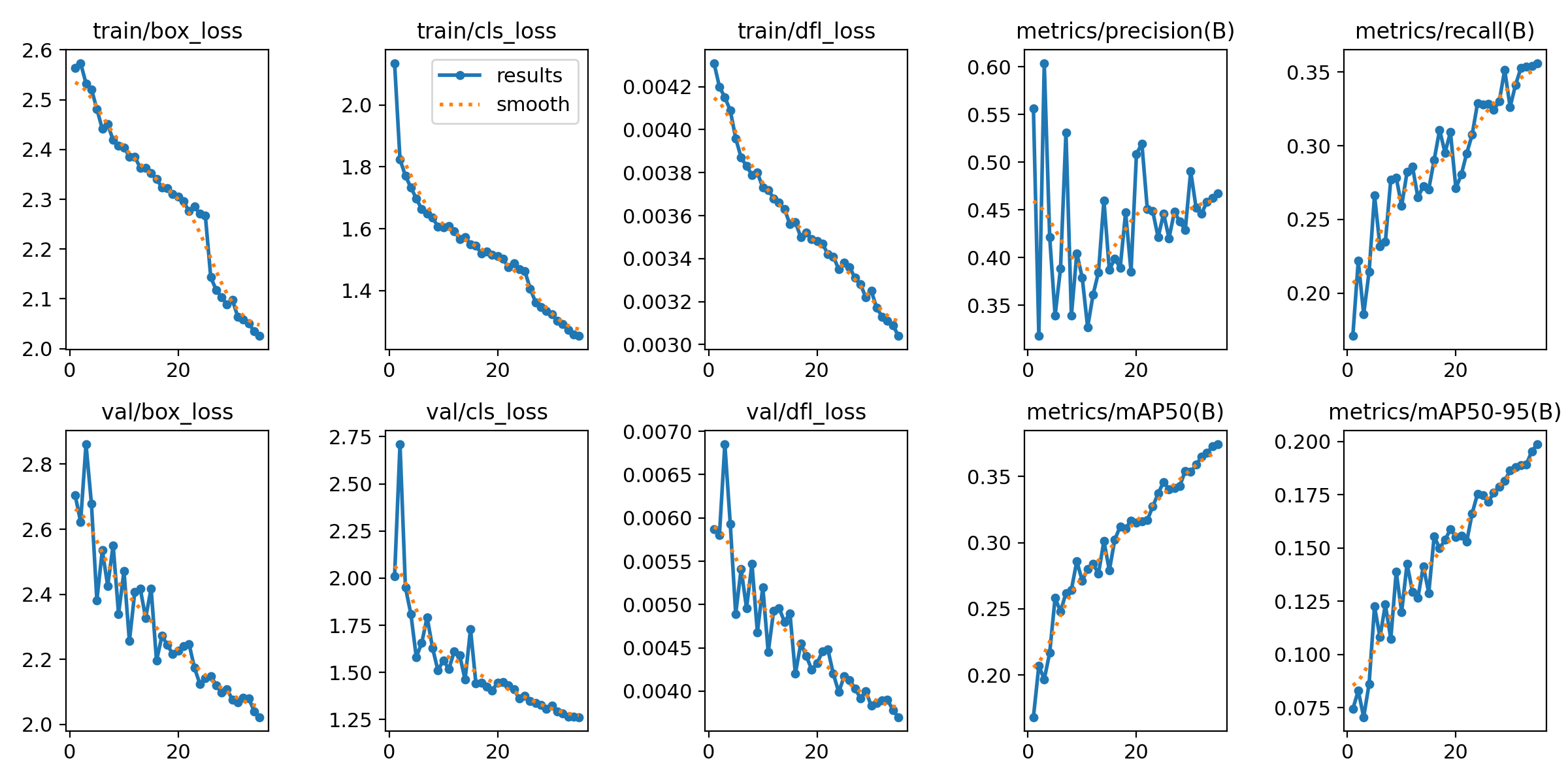
Overall Performance
The trained YOLOv8n model achieved a mAP50 of 33.2% on the validation set with precision of 44.7% and recall of 33.3%. Inference speed on CPU (Intel i7-10510U) averaged 22 FPS, meeting the real-time requirement.
While 33% mAP may seem low compared to standard detection benchmarks (COCO state-of-the-art exceeds 60%), this reflects the fundamental difficulty of the VisDrone dataset. Published results on VisDrone range from 30-45% mAP50, positioning this model in the competitive range for the nano variant.
Per-Class Performance
| Class | mAP50 | Precision | Recall | Instances |
|---|---|---|---|---|
| Car | 74.1% | 57.9% | 75.6% | 14,064 |
| Bus | 40.5% | 47.0% | 41.8% | 251 |
| Van | 34.3% | 49.0% | 32.7% | 1,975 |
| Motor | 33.8% | 47.6% | 33.2% | 4,886 |
| Pedestrian | 32.7% | 38.3% | 35.7% | 8,844 |
| Truck | 24.7% | 46.1% | 24.5% | 750 |
| Tricycle | 18.6% | 42.4% | 17.0% | 1,045 |
| Bicycle | 6.4% | 29.1% | 6.1% | 1,287 |
Key Observations
The model excels at detecting cars (74.1% mAP), which makes intuitive sense given they represent 46% of training data and are relatively large (median 50×30 pixels). Buses also perform well (40.5%) despite being rare, likely because their size (80×40 pixels) provides sufficient visual information.
Performance degrades dramatically for small objects. Bicycles achieve only 6.4% mAP with just 6% recall, meaning 94% of bicycles go undetected. The median bicycle size is 12×18 pixels, below the effective resolution threshold for this architecture. No amount of training data would overcome this physical limitation without architectural changes specifically designed for tiny objects.
The correlation between object size and detection accuracy is striking. Plotting mAP against median object area reveals a clear exponential relationship: objects below 400 pixels squared see precipitous performance drops.
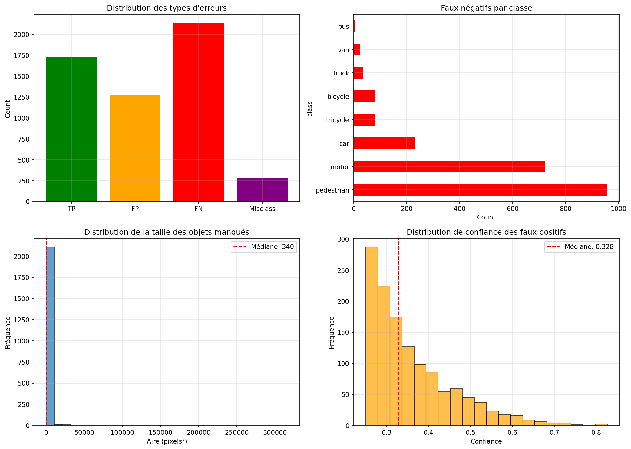
Failure Mode Analysis
To understand where the model fails, 100 validation images were analyzed, categorizing each prediction error:
False Negatives (2,132 total)
Objects present in ground truth but not detected by the model. Analysis reveals 67% of false negatives are objects smaller than 340 pixels squared. Pedestrians account for 955 false negatives (45%), followed by motors with 722 (34%). The model simply cannot extract sufficient features from these tiny instances.
False Positives (1,274 total)
Detections made by the model where no ground truth object exists. The median confidence score for false positives is 0.328, significantly lower than true positives (median 0.65). This suggests a clear separation: increasing the confidence threshold from 0.25 to 0.35 would eliminate approximately 40% of false positives while retaining most true detections.
Common false positive patterns include shadows misclassified as vehicles and image compression artifacts interpreted as pedestrians.
Misclassifications (279 total)
Correct localization but wrong class label. The most frequent confusion is between motor and bicycle (similar size and shape from above) and between van and truck (both rectangular vehicles). These errors are acceptable in many deployment scenarios where the distinction matters less than simply detecting a vehicle.
Poor Localization (702 total)
Correct class but IoU below 0.75. The model tends to predict bounding boxes slightly larger than ground truth, possibly a learned bias from the training objective which penalizes missed objects more than oversized boxes.
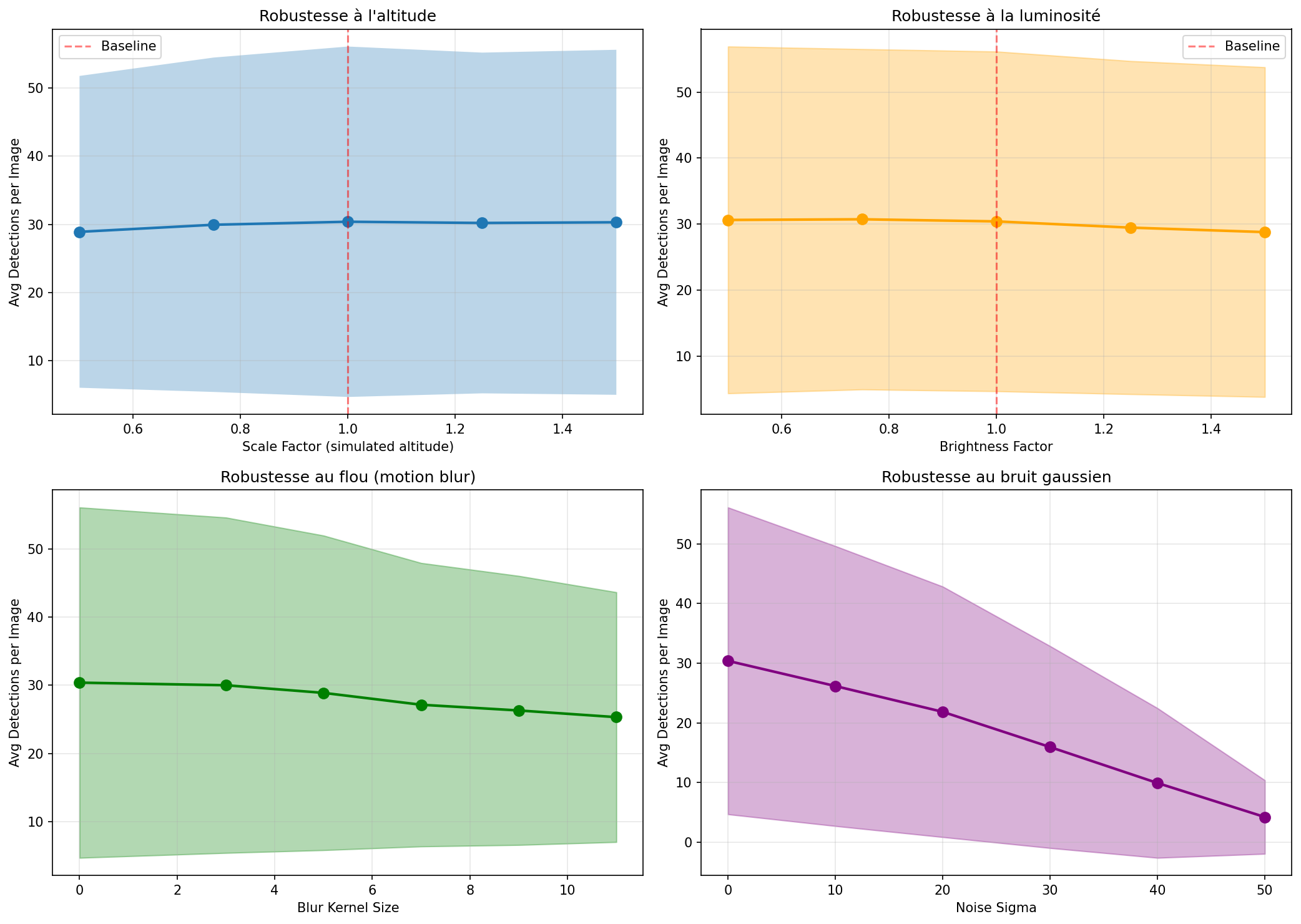
5- Robustness Testing Simulation
A production system must handle degraded conditions beyond the clean validation set. Four stress tests evaluated robustness.
Altitude Variation (Simulated Scaling)
Images were resized from 0.5× to 1.5× their original size to simulate altitude changes from 100m to 25m. Performance remained remarkably stable, varying only ±5% across the range. This validates the multi-scale training strategy and confirms the model generalizes across altitudes.
Brightness Variation
HSV value channel was multiplied by factors from 0.5 (dark) to 1.5 (bright). Performance degraded by approximately 8% at the extremes but remained acceptable within the 0.75-1.25 range. This indicates the model can handle daytime variation but would struggle in true night conditions without infrared imaging.
Motion Blur
Gaussian blur with kernels from 3 to 11 pixels simulated camera shake and fast motion. Performance dropped 17% at kernel size 11, equivalent to severe vibration or rapid panning. This suggests adding optical image stabilization or motion compensation preprocessing would significantly improve real-world performance.
Gaussian Noise
Random noise with standard deviation from 10 to 50 simulated sensor degradation and compression artifacts. Performance collapsed at σ=30, dropping 50% from baseline. This is the model’s critical weakness: deployment in rain, fog, or low-light conditions would require denoising preprocessing or a model specifically trained on degraded imagery.
Operational Recommendations
The model is production-ready for clear-weather daytime operations with stable camera platforms. Rain, fog, night, or high-vibration scenarios require additional preprocessing or architectural modifications. For defense and surveillance applications, this defines clear operational envelopes.
6- API Deployment
API Architecture
The trained model was wrapped in a FastAPI REST service providing two endpoints: /predict returns JSON bounding boxes and class labels, while /predict/annotated returns the image with visual annotations.
Each request is logged with structured JSON including request ID, image dimensions, detection count, per-class distribution, inference time, and throughput. This enables production monitoring and performance analysis.
Real-World Performance
Testing with 10 diverse validation images revealed median inference latency of 71.7ms and median throughput of 13.9 FPS. The distribution is tightly concentrated between 60-90ms with one outlier at 316ms caused by a large 1920×1080 image.
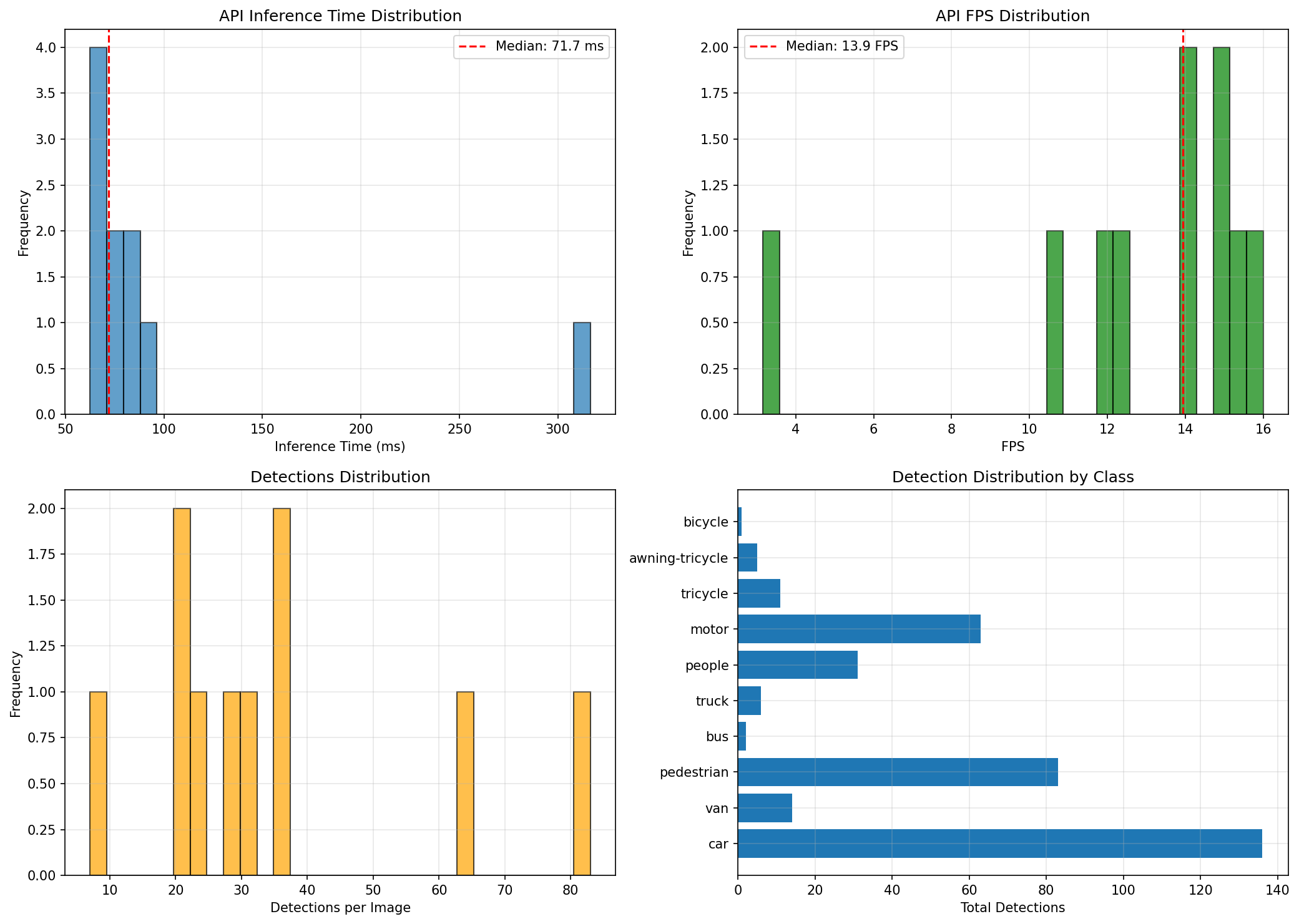
This consistency is critical for production deployment. Predictable latency allows proper request queue sizing and load balancing. The outlier behavior is explainable (large image) and can be mitigated with preprocessing to resize inputs before inference.
ONNX Export and Optimization
The PyTorch model was exported to ONNX format for deployment optimization. Counterintuitively, ONNX inference was slower on CPU (78ms vs 58ms for PyTorch). This occurs because PyTorch’s CPU backend is highly optimized for Intel architectures, while ONNX Runtime’s performance gains require specific hardware (NVIDIA TensorRT, Intel OpenVINO) or quantization.
The ONNX export remains valuable for future GPU deployment or edge device targeting, but for this CPU-based system, native PyTorch provides superior performance.
7- Hardware Integration: Reverse Engineering the Syma Z3 Pro
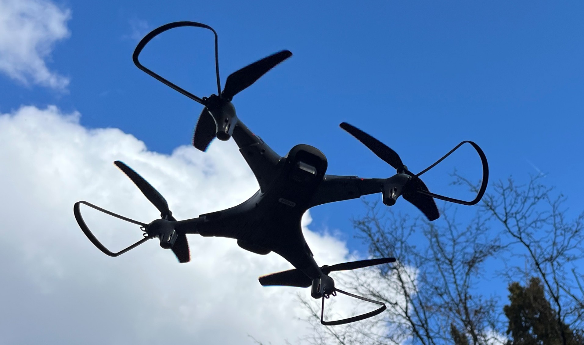
The Problem: No Documentation
The Syma Z3 Pro drone provides no public API documentation for accessing its video stream. The manufacturer’s mobile app displays live footage, but standard integration approaches all failed:
- Screen mirroring impossible: the phone must connect to the drone’s WiFi, preventing simultaneous connection to a computer network
- RTSP URLs tested without success:
rtsp://192.168.30.1:8080/live,rtsp://192.168.30.1:8081/live - HTTP endpoints returned no data:
http://192.168.30.1:8081/video
The goal was clear: extract the raw video stream directly from the drone without manufacturer support to enable real-time inference.
Network Reconnaissance
Port Scanning with nmap
Connecting a laptop directly to the drone’s WiFi hotspot and running a comprehensive port scan revealed the network topology:
PORT     STATE SERVICE
8080/tcp open  http-proxy
8081/tcp open  blackice-icecap
The MAC address fingerprint identified the hardware as a Shenzhen iComm Semiconductor chip (MAC: 50:9B:94:DA:82:4B), commonly used in low-cost consumer drones.
Binary Protocol Analysis
Establishing a raw TCP connection to port 8080 and examining the byte stream revealed a repeating pattern at the start of each data chunk:
0x00 0x00 0x00 0x01 0x67 ...
This four-byte sequence (00 00 00 01) is the H.264 NAL unit start code defined in the Annex B byte stream format specification. The presence of this signature confirmed the drone transmits raw H.264 video over TCP without any proprietary encapsulation, RTP framing, or authentication handshake.
The stream begins immediately upon TCP connection establishment, regardless of the client’s initial payload. This suggests a simple implementation: the drone’s firmware continuously encodes camera frames to H.264 and pushes them to any connected TCP client.
Stream Validation
Testing with ffplay confirmed the hypothesis:
ffplay tcp://192.168.30.1:8080
Output: H.264 High Profile, yuv420p color space, 640×384 resolution at 25 FPS. The stream was stable and continuous.
Real-Time Inference Pipeline Architecture
Direct integration with OpenCV proved problematic. Using cv2.VideoCapture on a TCP H.264 stream introduced excessive buffering (2-3 seconds delay) because OpenCV’s internal buffer management doesn’t account for live streaming constraints.
The solution required decoupling network I/O from frame processing through a multi-stage pipeline:
Stage 1: TCP Capture and Decode
An ffmpeg subprocess connects to the drone’s TCP port, decodes the H.264 stream in real-time, and retransmits it as MPEG-TS over UDP to localhost. This architecture provides several advantages:
- ffmpeg handles H.264 decoding with optimized native libraries
- UDP transmission prevents blocking when the Python process falls behind
- The fifo size parameter allows controlled buffer overflow behavior
Stage 2: Buffer Drain Thread
A dedicated Python thread continuously reads from the UDP socket using OpenCV, storing only the most recent frame in a thread-safe shared variable. This “drain” pattern prevents buffer accumulation when YOLO inference (slower than 25 FPS) cannot keep pace with the incoming stream.
Without this design, frames would queue up in the UDP buffer, creating increasing latency as old frames wait for processing. By discarding all but the latest frame, the system maintains minimal lag at the cost of skipping intermediate frames.
Stage 3: YOLO Inference and Tracking
The main loop reads the latest available frame, runs YOLOv8 detection every third frame (to maintain display framerate), and applies ByteTrack for persistent object IDs.
ByteTrack uses a Kalman filter to predict object positions between detections and matches predictions to observations using the Hungarian algorithm. This maintains identity even when objects temporarily disappear due to occlusion or the 1-in-3 inference schedule.
┌──────────────┐  TCP:8080   ┌─────────────┐  UDP:1234   ┌──────────────┐
│ Drone Camera │────H.264────▶│   ffmpeg    │───MPEG-TS──▶│ OpenCV Drain │
│ (Syma Z3 Pro)│              │  (decode)   │             │   (thread)   │
└──────────────┘              └─────────────┘             └──────┬───────┘
 640×384 @ 25fps               Subprocess                         │
                               Real-time                          ▼
                                                          ┌──────────────┐
                                                          │ YOLO26n      │
                                                          │ Inference    │
                                                          │ (every 3rd)  │
                                                          └──────┬───────┘
                                                                 │
                                                                 ▼
                                                          ┌──────────────┐
                                                          │  ByteTrack   │
                                                          │  (Kalman)    │
                                                          └──────┬───────┘
                                                                 │
                                                                 ▼
                                                          ┌──────────────┐
                                                          │   Display    │
                                                          │  27.5 FPS    │
                                                          └──────────────┘
Flight Test Results
Live testing with the drone in outdoor conditions yielded the following performance metrics:
| Metric | Value |
|---|---|
| Display FPS | 27.5 |
| Inference Latency (mean) | 62.4 ms |
| Frame Drop Rate | 0.0% |
| Total Frames Processed | 2,847 |
| Video Resolution | 640 × 384 |
| Effective Inference Rate | ~8 FPS (every 3rd frame) |
The zero frame drop rate indicates the buffer management strategy successfully handled the mismatch between the 25 FPS stream and ~8 FPS inference rate. The 27.5 display FPS (slightly above the stream’s 25 FPS) confirms minimal latency in the pipeline.
Session Recording
Each flight session is automatically recorded as an MP4 file with annotated bounding boxes and tracking IDs overlaid. The recordings preserve all detections for post-flight analysis and provide training data for iterative model improvement.
8- Field Validation & Experimental Protocol
[Work in progress]
9- Bonus: Counter UAS Interceptor Simulation
Beyond detection, the system demonstrates feasibility for Counter-UAS (C-UAS) applications through a physics-based interceptor trajectory simulation built from the ground up.
System Architecture:
The simulation implements a complete engagement loop with realistic dynamics:
- Threat Model: Incoming missiles with five trajectory profiles (linear pursuit, ballistic arc, sinusoidal weaving, spiral corkscrew, zigzag hard-breaks) plus proximity-based active evasion when interceptors close within a configurable range
- Sensor Fusion: 6-state Kalman filter (position + velocity) tracks noisy radar measurements with configurable process noise (σ=5 m/s²) and measurement noise (σ=15 m)
- Guidance Laws: Three classical homing strategies — Proportional Navigation (PN), Pure Pursuit (PP), and Lead Pursuit (LP) — with saturated acceleration commands
- Multi-Engagement: Supports N vs. N scenarios (up to 6 simultaneous missile/interceptor pairs) with shared radar picture and independent tracking per pair
Proportional Navigation Implementation:
The core guidance law computes lateral acceleration proportional to the line-of-sight rotation rate:
$$\vec{a}_{\text{cmd}} = N \cdot V_c \cdot (\vec{\omega} \times \hat{R})$$
Where:
- $N$ = Navigation constant (typically 3-5, configurable via
--Nflag) - $V_c$ = Closing velocity (negative radial velocity component)
- $\vec{\omega}$ = Line-of-sight angular velocity vector $\frac{\vec{R} \times \dot{\vec{R}}}{|\vec{R}|^2}$
- $\hat{R}$ = Unit vector from interceptor to target
This law ensures the interceptor leads the target appropriately, nulling the line-of-sight rate to achieve collision.
3D Visualization:
The simulation renders in real-time using PyVista (interactive 3-D scene):
- Color-coded trajectories per engagement pair
- Kalman filter estimate overlay
- Telemetry HUD displaying range, time-to-go, and engagement status
- Explosion effects at intercept points
- Post-analysis plots: range convergence curves, altitude profiles, intercept timing markers
Linear missile attack
 Multiple missile attacks with spiral trajectory and counter-uas avoidance
 Multiple missile attacks with sinusoidal trajectory
Conclusion
Limitations and Improvements
Small object performance remains the fundamental constraint. Objects below 20×20 pixels are essentially undetectable with this architecture. Solutions require either specialized tiny object detectors (SAHI tiling approach, feature pyramid refinement) or higher-resolution input (computationally expensive, requires better camera hardware).
Weather robustness is insufficient for all-weather operation. The 50% performance drop under simulated noise (σ=30) indicates the model would struggle in rain or fog. Either preprocessing with learned denoisers or training on degraded data is necessary.
Tracking through occlusion occasionally loses IDs when objects disappear behind obstacles for extended periods. More sophisticated trackers with appearance-based re-identification (DeepSORT with ResNet features) would improve identity persistence at the cost of additional computation.
WiFi range limitation of approximately 30 meters line-of-sight restricts operational deployment. Upgrading to 5 GHz WiFi, adding directional antennas, or implementing onboard processing would extend viable range.
Potential applications
For defense, surveillance, or autonomous systems applications, this work provides a realistic baseline with clearly defined operational envelopes (clear weather, daytime, moderate altitude, 30m WiFi range) and a concrete roadmap for addressing current limitations through hardware upgrades, architectural improvements, and dataset expansion.
The code, trained models, and documentation are available on GitHub for reproduction and extension.
Python · PyTorch · Ultralytics YOLO · FastAPI · OpenCV · ffmpeg · Network Analysis · Protocol Reverse Engineering · ByteTrack · Computer Vision